Build a 3D Coastal Model (Level 2 Step-by-Step Guidance)
- Kester Scandrett
- Linh Nguyen
- Duy Pham
1. Introduction
This tutorial document will provide a guideline on how to set up a coastal hydrodynamic model by using the EFDC+ Explorer (EEMS). It will cover the preparation of the necessary input files for the EFDC model and visualization of the output by using the EFDC+ Explorer Software.
The data used for this tutorial are from Tra_Khuc Estuary in Vietnam. All files for this tutorial are found in Data folder downloadable from the EEMS Website.
Before going to each session, let us first introduce the EE main form in order to better understand our explanation hereafter. Figure 1 is the main form of EFDC+ Explorer or EE User Interface. The functions of individual icons are described in Model Control Form.
Figure 1. EFDC+ Explorer main form.
2. Create a New Grid
This section will provide guidelines on how to create a new simple gird with EFDC+ Explorer. For a complicated grid, users are recommended to use specialized grid generation software such as Grid+.
Tra_Khuc Estuary in Quang Ngai province, Vietnam is chosen as the example of building a 3D coastal model.
The gird generation process includes the following steps:
1.Open EE
2.Click on icon New Model on the main menu of EE interface.
3. In Grid Tool, select Import Grid from Files and click Import Grids button. Users should choose Grid type as Grid+ and then click Browse button to select the grid file name as "Tra_Khuc.cvl" in Grid folder as shown in Figure 2. On the other hand, EE also supports users to import various formats of grid files with the option Grid type.
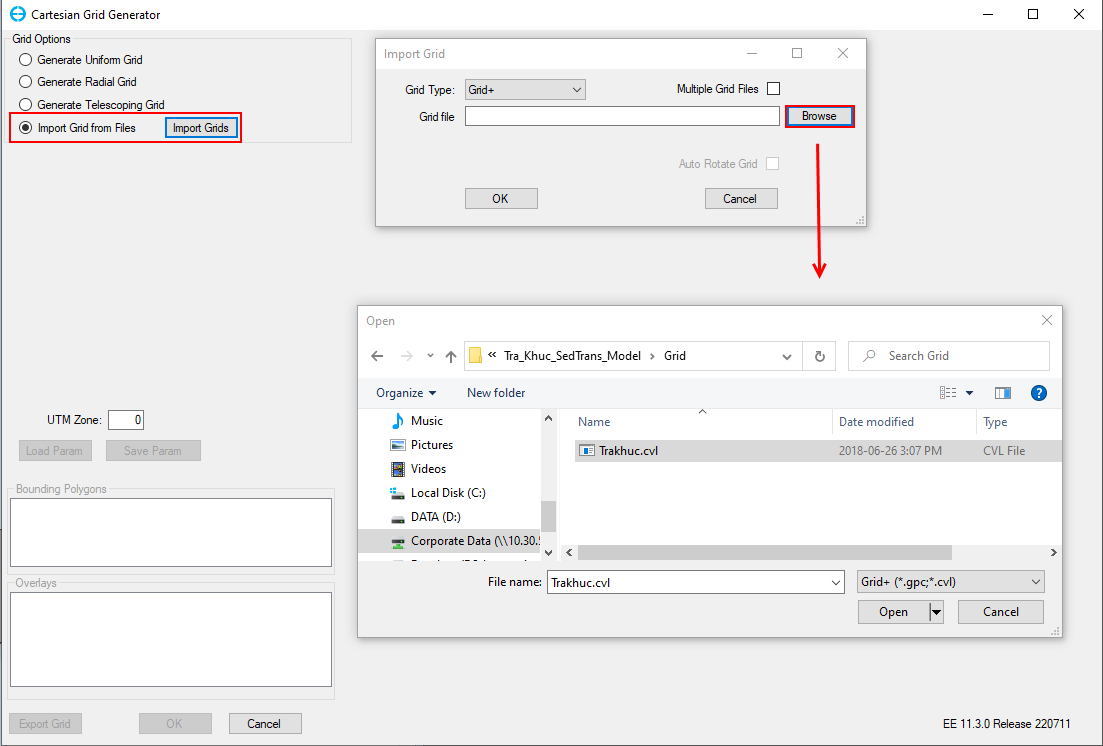
Figure 2. Import grid file.
4. Set UTM Zone is 49 and then click OK to load the grid in Figure 3.
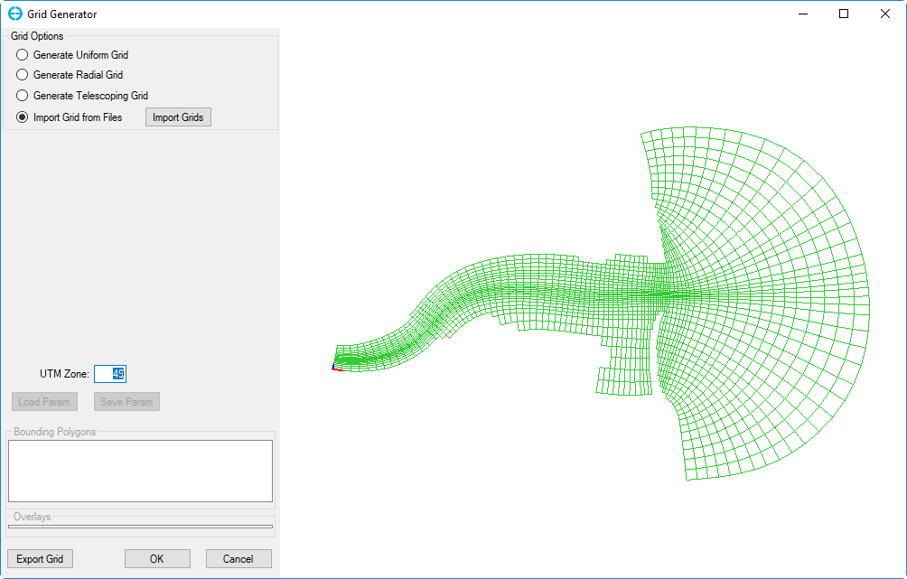
Figure 3. Load grid file.
5. Save the model by selecting this button  in the main toolbar and create a new directory (as shown in Figure 4)

Figure 4 New model saved.
3. Assigning the Initial Conditions
This section will show how to assign the initial conditions such as the bathymetry, and water level.
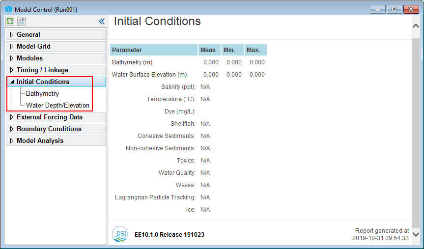
Figure 5. Assigning initial conditions.
3.1 Assigning the Bathymetry
- Right mouse click (RMC) on Bathymetry in the Model Control tab. A popup Bathymetry tab will appear as presented in Figure 6, click Assign button.
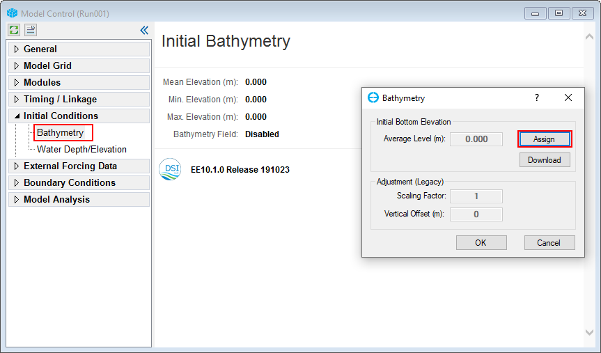
Figure 6. Initial bathymetry.
2. The Apply Cell Properties via Polygons: Bottom Elevation form appears, select options Only grid cells inside polygons, Scatter (XYZ) data, Centroid Interp as a polyline file is used to define the area to assign the bathymetry data.
3. For Polygon Files, users should click Add File button to browse the file "Domain.p2d" in the Bathymetry folder Figure 7 and Figure 8.
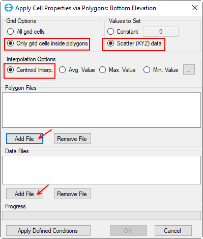
Figure 7. Apply Cell Properties via Polygons: Bottom Elevation form.
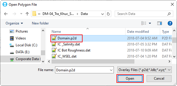
Figure 8. Add polygon file.
4. In this example, Scatter (XYZ) data is recommended to select to set the data values for bathymetry. In Scatter Data Files, users should click Add File to browse to the bathymetry data named "Bathymetry.dat" in the Bathymetry folder as shown in Figure 9.
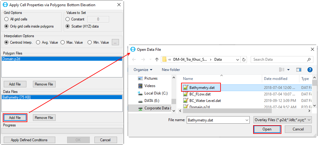
Figure 9. Adding bathymetry data file.
5. There are a number of options for users to modify the assigned. In this case, users can select Centroid Interpolation in the Interpolation Options. Click Apply Defined Conditions to apply all the settings before. A pop-up message will appear to inform the modified cell information, click OK (Figure 10).
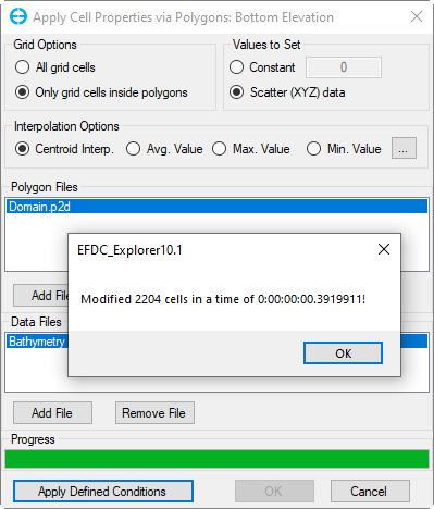
Figure 10. Results of assigning the bathymetric condition.
Note that you can also obtain the bathymetry data from an online source. See the page (Online Download Data Feature in EEMS10)
3.2 Assigning the Depth/Water Surface Elevations
The next steps show the way to assign the initial depth or water surface elevations.
- RMC on Water Depth/Elevation in Model Control tab. A popup Water Depth/Surface Elevation tab will appear as presented in Figure 11, click Assign Elevation button.
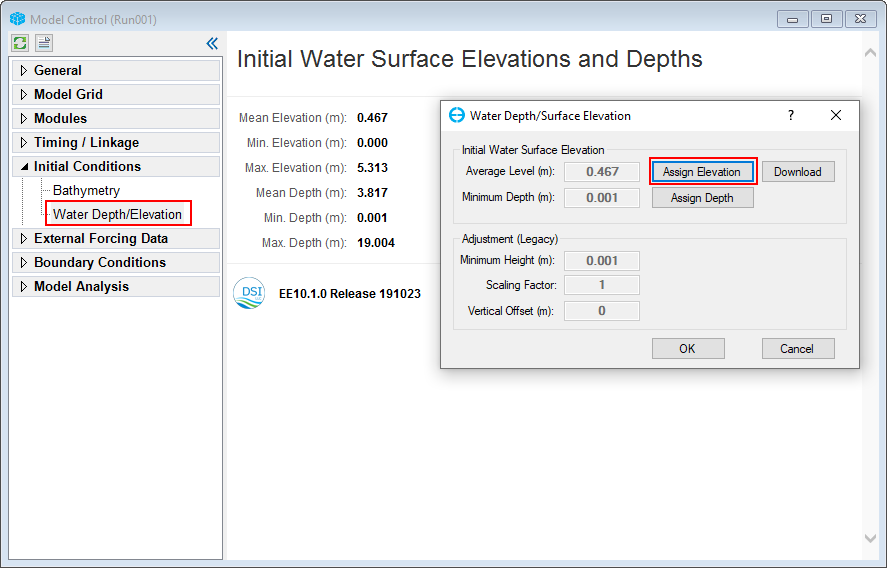
Figure 11. Assign initial water surface elevation.
2. A polyline file is used to define the area to assign the bathymetry data. In Grid Options, select option Only grid cells inside polygons. In Polygon Files, users should click Add File button to browse the file "Domain.p2d" in Bathymetry folder. (Figure 12).
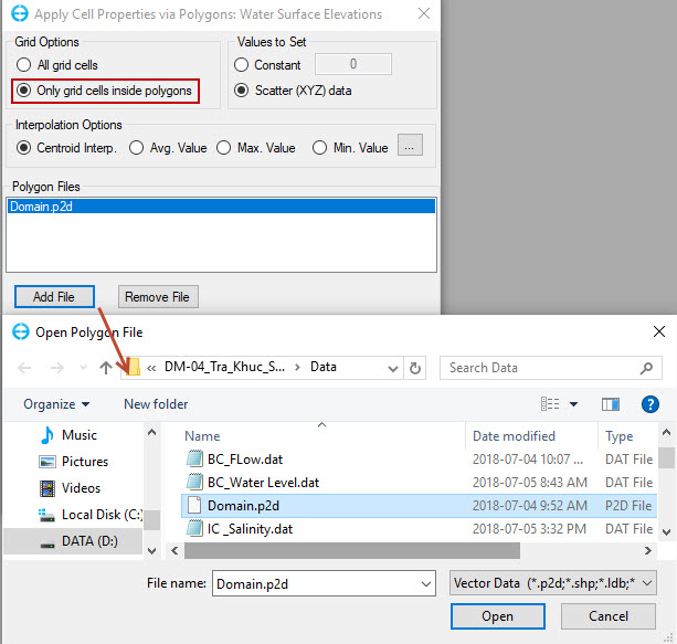
Figure 12. Add polygon file to assign water surface elevations.
3. In this example, Scatter(XYZ) data is recommended to select to set the data values for water surface elevations. In Scatter Data Files, users should click Add File to browse to the water elevation data named "IC_WSEL.dat" in the Boundaries folder as shown in Figure 13.
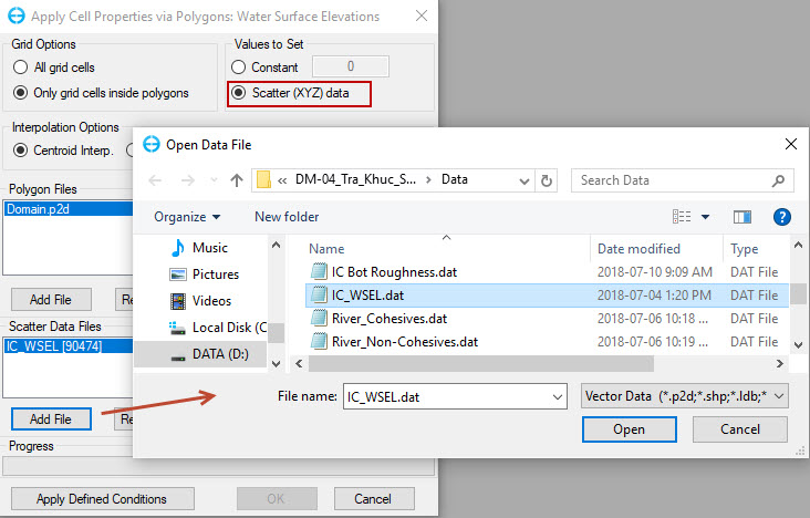 Figure 13. Add water surface elevation data.
4. There are a number of options for users to modify the assigned. In this case, users can select Centroid Interpolation (Figure 14) in the Interpolation Options.
5. Next, click Apply Defined Conditions to apply all the settings before. A pop-up message will appear to inform the modified cell information, click OK (shown as Figure 14).
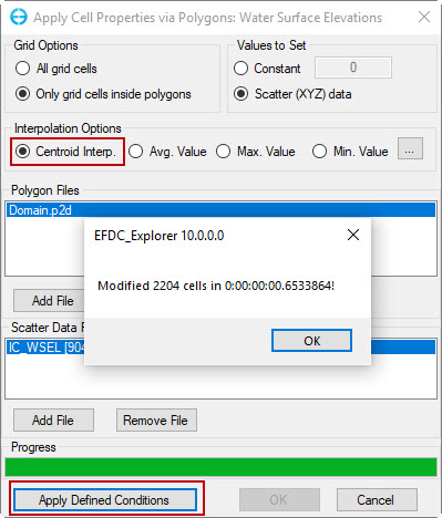
Figure 14. Results of assigning the water surface elevations.
4. Assigning the Boundary Conditions
The main aim of this section is to show how to prepare for the boundary conditions and assign them to the model cell configuration. In this coastal case, there are two flow boundaries; one is river discharge from the upstream and the other is tidal level. Thus, users should prepare two time series of inflow and tidal level boundaries for this particular case. In order to set a boundary time series the steps outlined below should be taken.
4.1 Preparing the Flow Boundary.
1.In Model Control, users should click on External Forcing Data tab, then RMC on Flow and select Add New Data Series (see Figure 15).
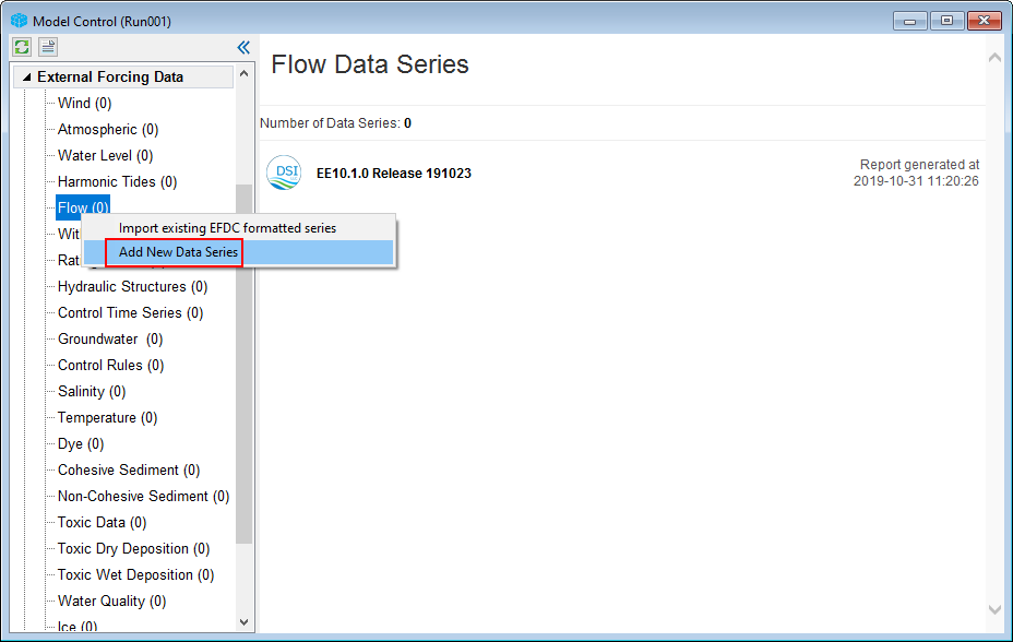
Figure 15. Assigning flow boundary conditions.
2. In order to add a new boundary data series, click Add New button and type the series name as "River". LMC on Import data from files by selecting this button  and click Import Series as shown Figure 16.
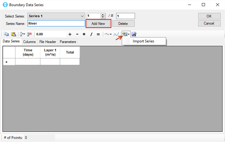
Figure 16. Add new boundary data series.
3. For ASCII Data Import, users should browse to "BC_Inflow.dat" file in the Boundaries folder and click Open to import file. Check the Date Format as EE DAT or WQ Data and Header Rows to Skip before clicking OK ( illustrated in Figure 17).
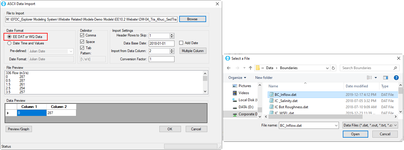
Figure 17. Import flow boundary.
4. Users can select which layer they want to assign value to in the Import Data tab. In this example, please check -1 to assign the same value for all layers and click OK. (Figure 18).
5. A pop-up window will appear to inform that data is imported successfully and click OK.
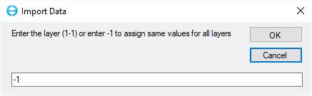
Figure 18. Import data.
6. To view the data series plot, users could check View Series button in the toolbar.
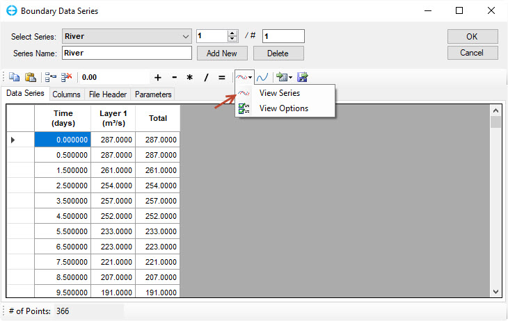
Figure 19. View data time series plot.
7. The time series plot will be shown as Figure 20. EE10 also supports users to edit, and export the time series plot. Please check the toolbar and the user guide for more functions.
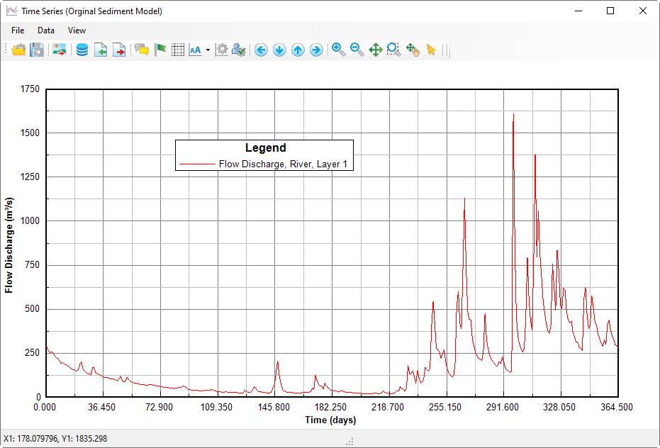
Figure 20. Time series plot.
4.2 Preparing the Tidal Level Boundary.
- RMC on Water Level and select Add New Data Series Figure 21.
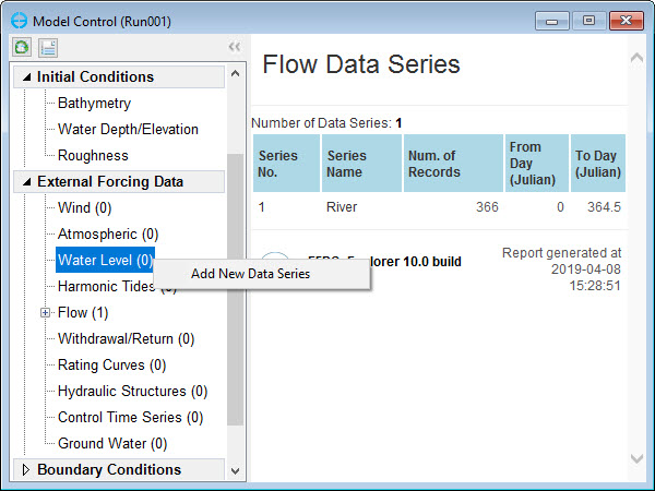
Figure 21. Preparing the tidal level boundary.
2. Click on Add New to insert a new data series and name it "Tides" in Series Name. Browse to the "BC_Water Level.dat" file in the Boundaries folder and click Open to import data file (shown Figure 22).
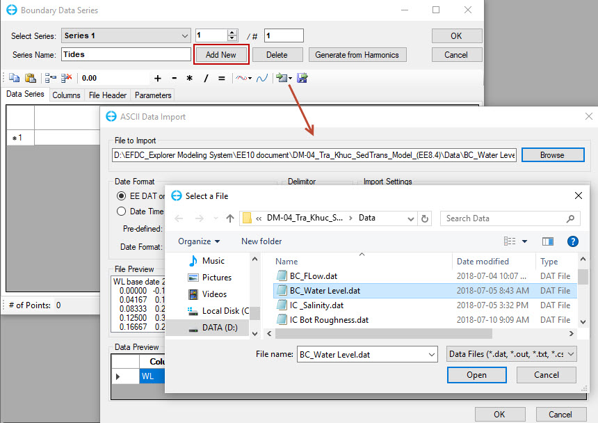
Figure 22. Import water level time series.
3. Check the Data Format as EE DAT or WQ Data and select Header Rows to Skip as 1 before clicking OK. Then, users should enter -1 to assign the same values for all layers (See Figure 23). After clicking OK, a pop-up message will appear to inform that data was imported.
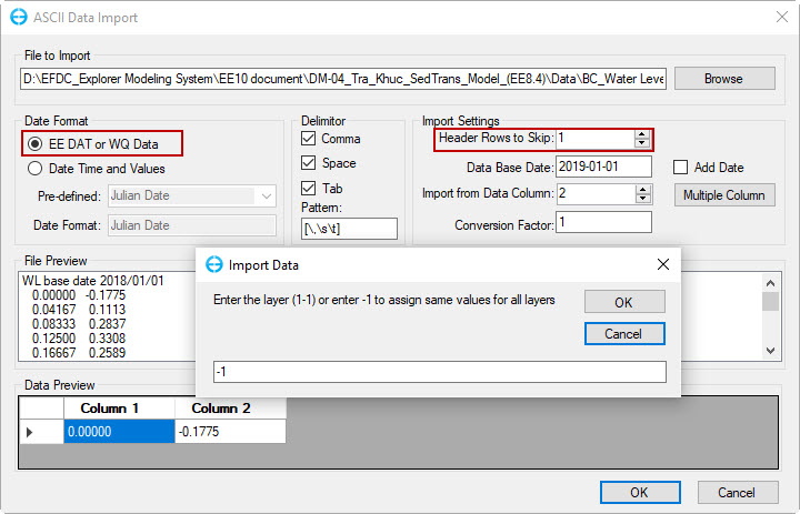
Figure 23. Selected the data format to import.
4. Select View Series as this button  to visualize the data time series as shown in Figure 24 below.
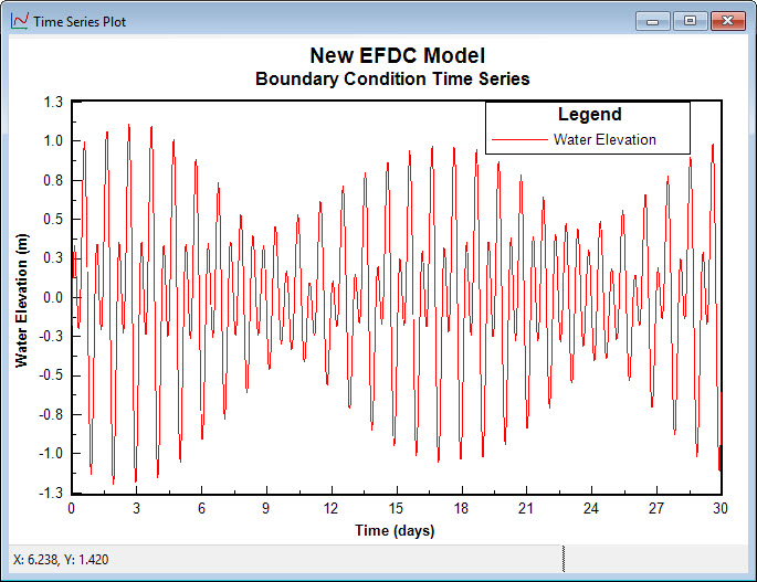
Figure 24. Water elevation time series plot.
4.3 Assigning Time Series to the Boundary Location Cells.
When all required boundary time series are prepared the next step is to assign those boundary time series to the model cells.
4.3.1 Assigning the Flow Boundary
In order to assign the flow boundary, the following steps should be taken. Figure 25 shows the location of inflow and tidal level at the open boundary for the Tra_Khuc model case.
- Click to the 2DH View icon
 on the main form.
 - In View Layer Control, turn on the Model Grid layer and turn on the editing mode of the Boundaries Layer
 by clicking the pencil icon shown as Figure 25.
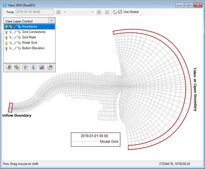
Figure 25. Locations of inflow and open tidal boundaries.
3. Click on Selection Tool  in the main toolbar and then select Line Crossing
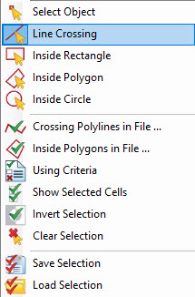
Figure 26. Line crossing.
4. Use line crossing to select all the cells at the inflow boundary location in Figure 26. Then, RMC on a selected cell and choose Add New Boundary Group (see Figure 27).
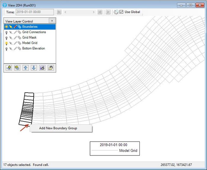
Figure 27. Add a new inflow boundary group.
5. Enter the inflow boundary group as "River" and select boundary group type as "Flow Boundary" ( as Figure 28).
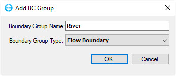
Figure 28. Set up inflow boundary.
6. Figure 29 shows flow boundary conditions tab, users should check the flow table as "River" and set it for all by clicking All button. A pop-up message will show to inform that 17 cells have been changed, then click OK.
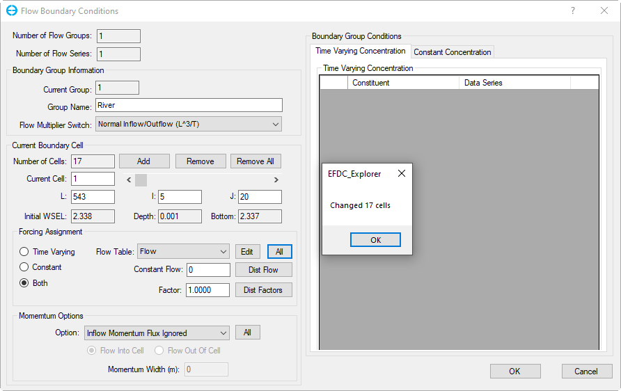
Figure 29. Assign boundary conditions for all selected cells.
7. The inflow boundary is now assigned to all selected cells as shown in Figure 30.
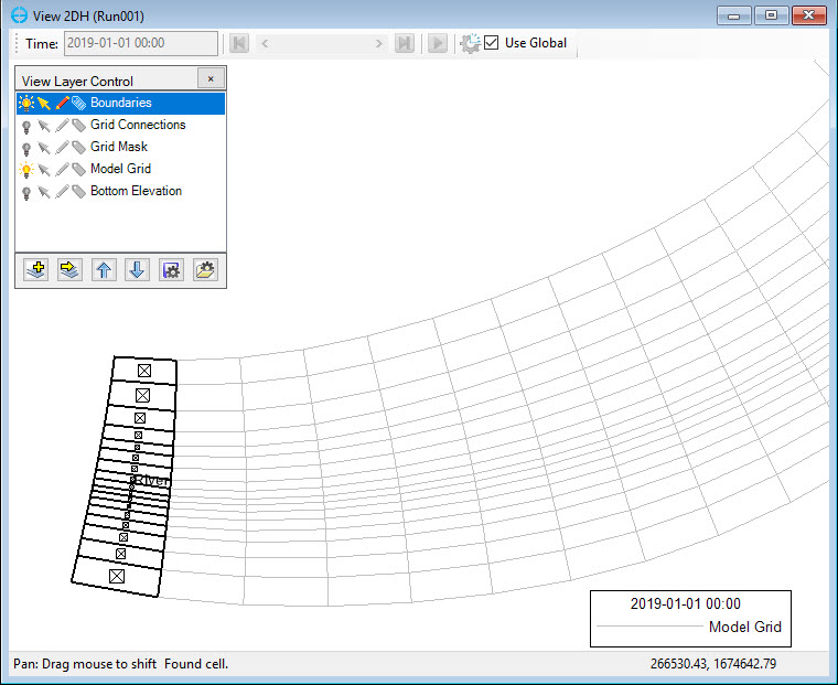
Figure 30. Upstream boundary cells assigned.
4.3.2 Assigning Tides Boundary
In order to assign the tides boundary, the following steps should be taken:
1.Click to the 2DH View icon  on the main form.
2. In View Layer Control, turn on the Model Grid layer and turn on the editing model of the Boundaries Layer by clicking the pencil icon shown as Figure 25.
3. Clicking on Selection Tool in the main toolbar and then select Inside Polygon as Figure 31.
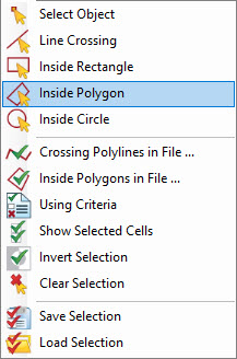
Figure 31. Select inside polygon.
4. Draw a polygon that can cover all the cells at the tides boundary location in Figure 32.
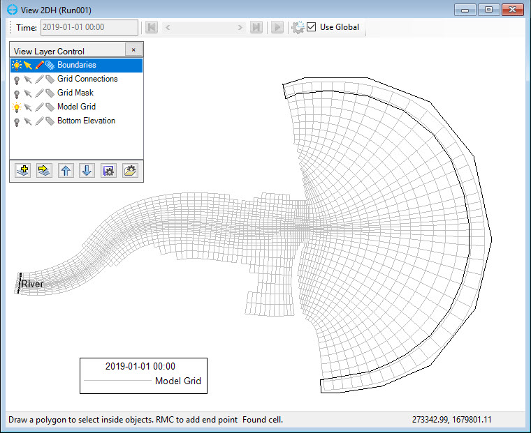
Figure 32. Draw a polygon to assign tides boundary.
5. To assign the tides boundary group, users should RMC on a selected cell and click Add New Boundary Group as Figure 33.
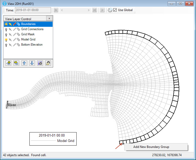
Figure 33. Add new tides boundary group.
6. Enter the Boundary Group Name, "Ocean" and select the appropriate boundary type as Figure 34. In this case, the river flows to the east, so choose " East Open Boundary".
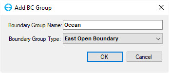
Figure 34. Set up tides boundary.
7. Select level data time series that were created earlier, "Tides" as shown in Figure 35. Next, click All button to assign tides to all cells. The number of changed cells will be informed and click OK.
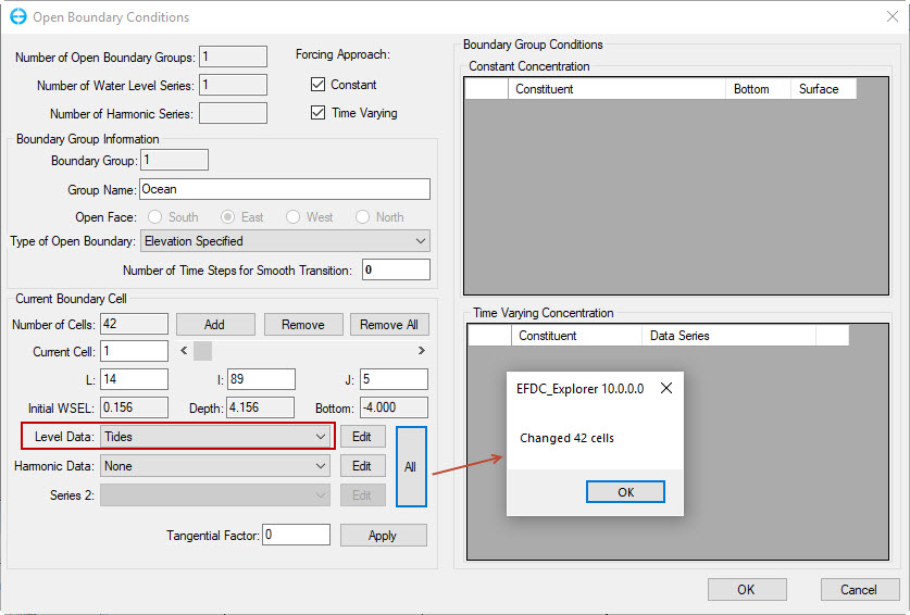
Figure 35. Assign tide flow boundary.
8. The tides open boundary is now assigned for all selected cells as presented in Figure 36.
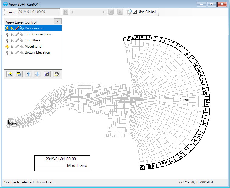
Figure 36. Tides boundary cells are assigned.
5. Hydrodynamics Model
- Back to the main tab, select Windows in the toolbar and click to Model Control, or select Model | Show Active Model from the main menu.
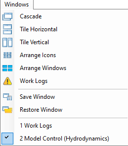
Figure 37. Use the Windows option to return to the Model control tab.
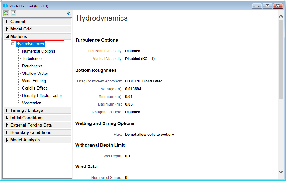
2. In Modules sub-main tab, click + to expand Hydrodynamics tab, all sub-tabs of Hydrodynamics will be shown as Figure 38. The users need to RMC on each sub-tab to adjust option settings.
 .
.
Figure 38. Hydrodynamic options setup.
3. Set Roughness
RMC on Roughness. A popup Bottom Roughness tab will appear as presented Figure 39, click Assign button.
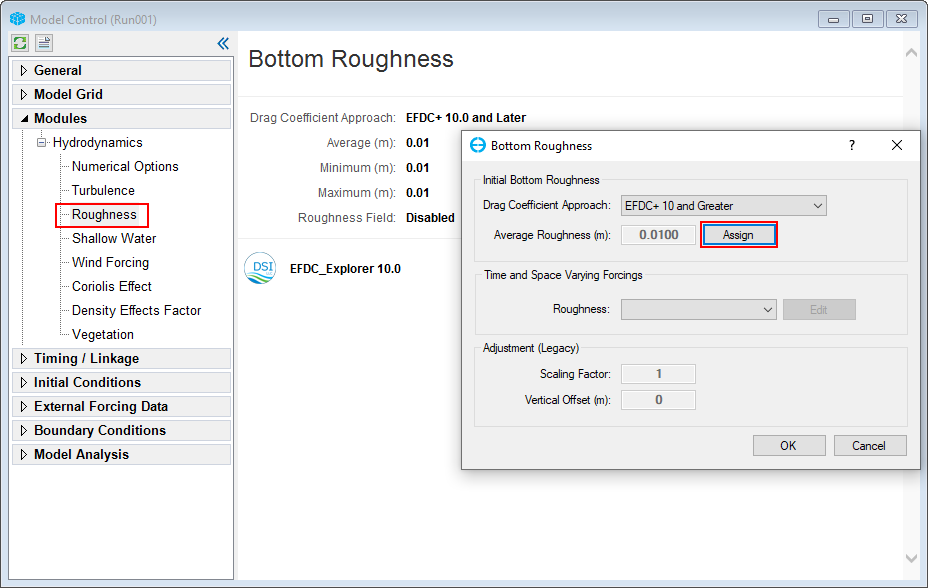
Figure 39. Assign bottom roughness.
For Grid Options, select option Only grid cells inside polygons. In Polygon Files, users should click Add File button to browse the file "Domain.p2d" in the Bathymetry folder (Figure 40).
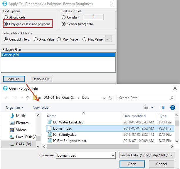
Figure 40. Load polygon file.
Select Scatter (XYZ) data to set the data values for the bottom roughness. In Scatter Data Files, users should click Add File to browse to the bottom roughness data named "IC_Bot_Roughness.dat" in the Boundaries folder as shown in Figure 41.
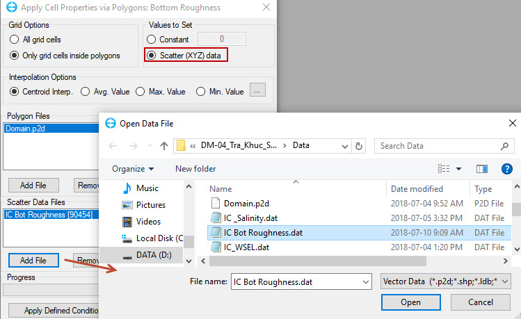
Figure 41. Load bottom roughness data.
There are a number of options for users to modify the assigned. In this case, users can select Centroid Interpolation (Figure 42) in the Interpolation Options.
Then, click Apply Defined Conditions to apply all the settings before. A pop-up message will appear to inform the modified cell information, click OK (shown as Figure 42).
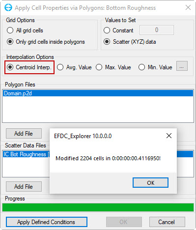
Figure 42. Results of assigning bottom roughness.
4. Setting Wetting and Drying
The Shallow Water settings are important in coastal simulations. In this case, users should set the Shallow Water Options as in Figure 43.
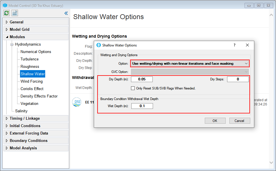
Figure 43. Wetting and Drying setting for the model.
5. Setting Turbulence
RMC on Turbulence sub-tab, in the Turbulence Options, select Turbulent Diffusion to set turbulence diffusion. Select options as "Smagorinsky" and click OK (as shown in Figure 44).
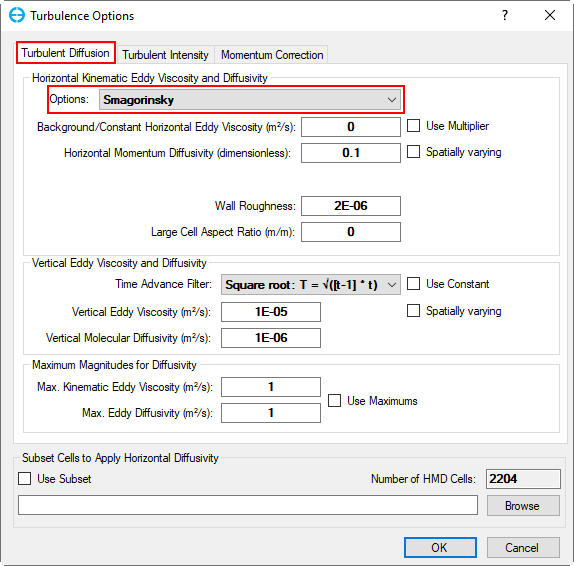
Figure 44. Turbulence Diffusion Settings.
6. Salinity Model
6.1 Activate Salinity Modules
In the Model Control form, RMC on Modules to open the EFDC+ Modules window. In the EFDC+ Modules, check the Salinity checkboxes and then click OK (as shown in Figure 45). The Salinity item will then be added under Modules.
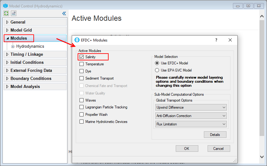
Figure 45. Active EFDC+ modules form.
6.2 Salinity Module Setting
6.2.1 Salinity Initial Condition
From the Model Control form, RMC on the Salinity module sub-tab under the Modules tab; a list of options will appear for the user to select, as shown in Figure 46 below.
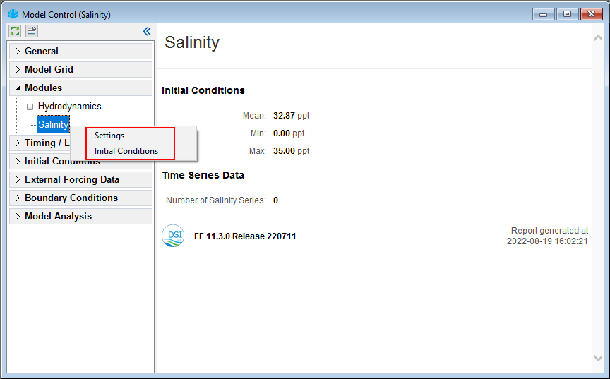
Figure 46. General salinity module setting options.
After clicking Initial Conditions, form of Initial Water Column Salinity Concentration will appear as shown in Figure 47.
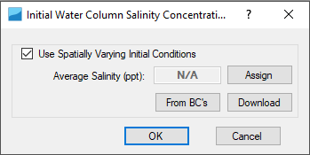
Figure 47. Salinity initial conditions.
After clicking on Assign button, the Apply Cell Properties: Salinity form will appear. In this form, which is shown in Figure 48 below user should follow these steps:
- In the Values to Set frame, select From Scatter (XYZ) data
- In the Data Files frame, click on the Add File button to browse to the salinity time series file name “IC_Salinity.dat”
- Click on Apply Defined Conditions to assign salinity initial condition. This sets the salinity data for the model.
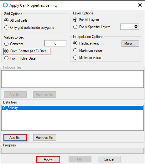
Figure 48. Apply cell properties for salinity.
6.2.2 Assign Boundary Concentration
Returning to the Model Control form and do the following steps as shown in Figure 49 to assign the salinity to boundary groups.
- Expand the Boundary Conditions tab on the left side of the screen; then expand the Water Level group; RMC on the Ocean group; then select Edit Boundary Group to open the Open Boundary Conditions
- In the Boundary Group Conditions frame of the Open Boundary Conditions form, under the Constant Concentration tab, set the salinity concentration of the bottom and surface layer as 35ppt
- Click the OK button to save the settings.
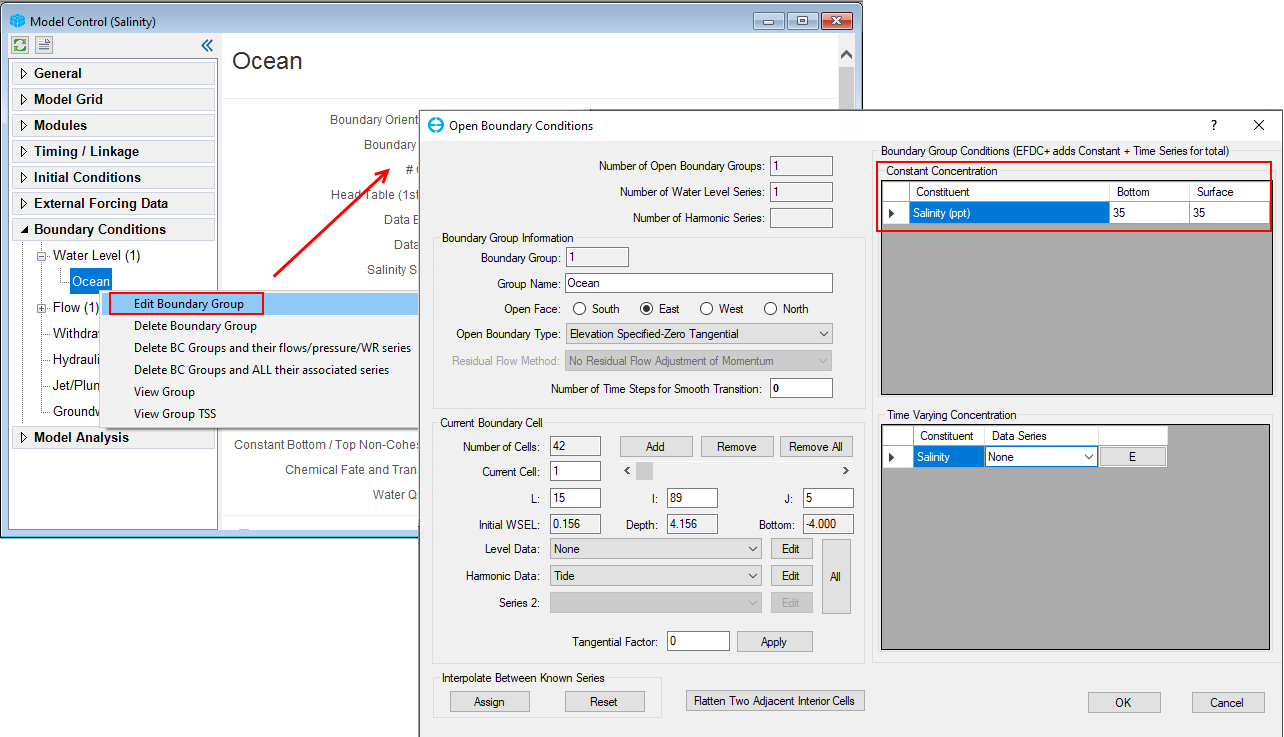
Figure 49. Set the constant salinity in the ocean boundary.
7.Setting Vertical Layers
The model is ready for running a test now. Normally a model is run for one vertical layer for initial calibration. It is also possible to add more vertical layers by the following steps (as shown in Figure 50):
- RMC on Grid in the Model Grid.
- Select Standard Sigma
- Enter the number of vertical layers into the box (# Layers). For Tra_Khuc case, set vertical layers to 5 layers and then click OK to save the setting.
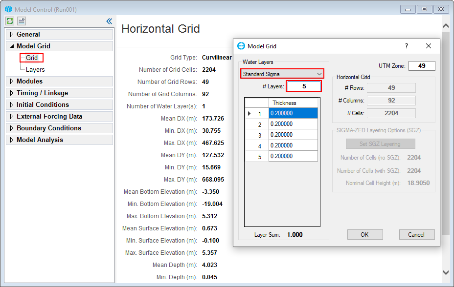
Figure 50. Setting the vertical layers.
8. Model Timing
The final step is to set the model simulation time and model time steps.
- In the Timing / Linkage, RMC on Timing. Enter the duration of starting/ ending the simulation as Figure 51. Note that the boundaries time series should be always covered in this simulation duration period. Otherwise, the model will not able to run.
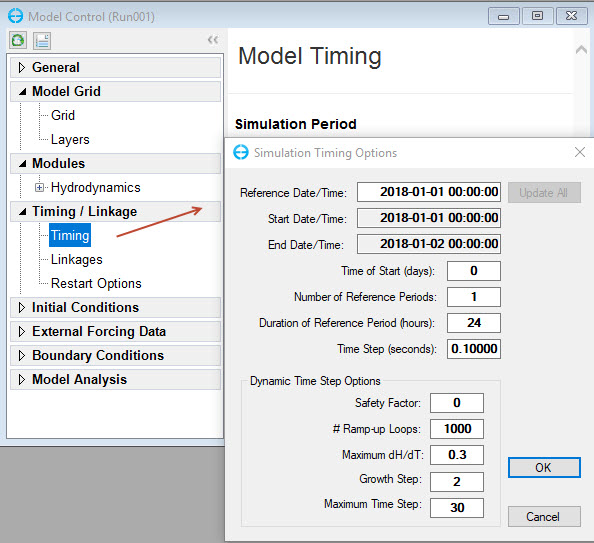
Figure 51. Setting the model run time.
2. RMC to Linkages and select the EFDC+ Explorer Linkage tab to set the frequency of the output of the EFDC results. Setting this to 15 minutes means that EFDC will save the output every 15 minutes for the display of the model results in the EE (Figure 52). Click OK button
Note that, the smaller output frequency will create a larger output file.
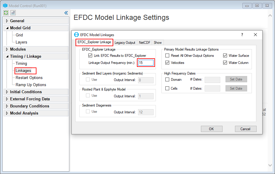
Figure 52. Setting Linkage Output Frequency.
9. Running EFDC+
Back to the main form, click this button  to run the model. Browse to the EFDC+ executable file and select the updated executable file as shown in Figure 53. Click Run EFDC+ button to run model.
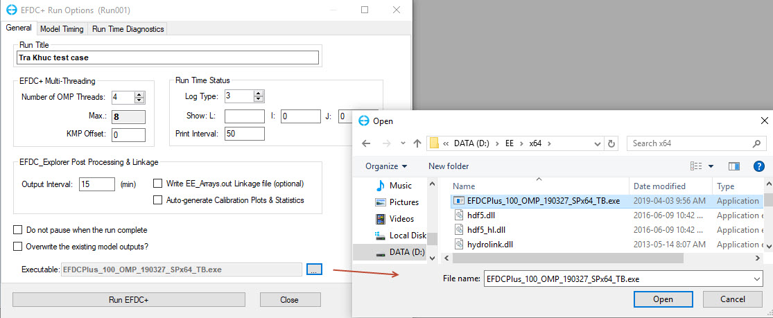
Figure 53. Run EFDC settings.
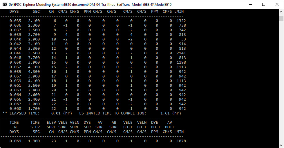
Note
Note that users can hit any characters on the keyboard to pause the simulation and check the model results. If they want to exit the simulation hit the same key if they want to continue running then hit any other key.
10. Visualizing the Model Output
This session will show how to view the model simulation results.In general, users can access the main form to click 2DH View button to view the model simulation results.
- In Layer Control, click Add button to add a New EFDC View Layer . The users should see the 2DH View Options window with Primary Group and Parameter to display (as shown in Figure 55), after selecting the parameter the users should click Add button to add the layer in 2DH View.
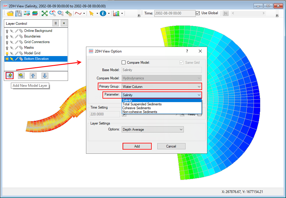
Figure 55. Parameter visualization.
2. Figure 52 is an example of showing the salinity results. Similarly, EE is able to support the visualization of other model parameters.
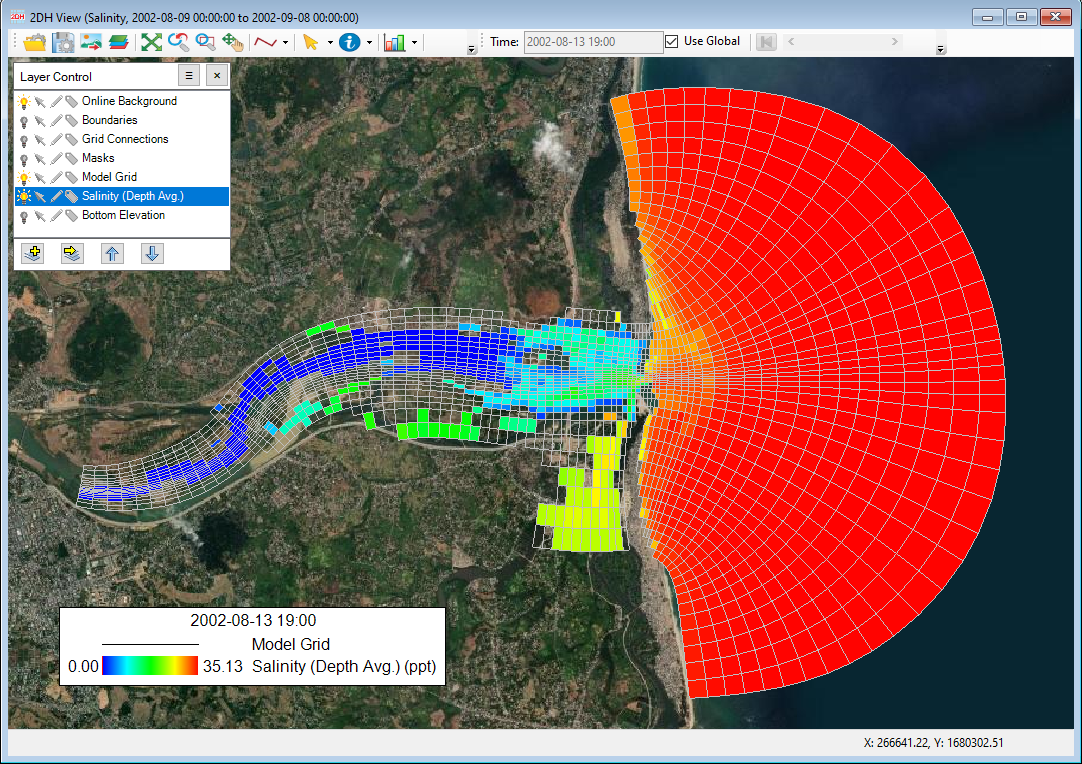
Figure 56. Velocity vector visualization.
Please refer to the “EFDC+ Explorer User’s Manual” for more information on EE capabilities.