Building a 2D Lake Water Quality Model (Level 2 Step-by-Step Guidance)
1. Introduction
Lake Thonotosassa is the largest natural freshwater lake in Hillsborough County covering an area of 849 acres (3.44 km2) (Hillsborough County Water Atlas). The lake is fed by Baker Creek at the southeastern end of the lake and water flows out through Flint Creek on the northeastern end to the Hillsborough River (Figure 1). This guidance document carries on from the hydrodynamic model introduced in Build a 2D Lake Model (Level 1 Step-by-Step Guidance). The model files are contained in the Demonstration Models of the Resources page folder file (1.14 Lake T Hydrodynamic and WQ Model).
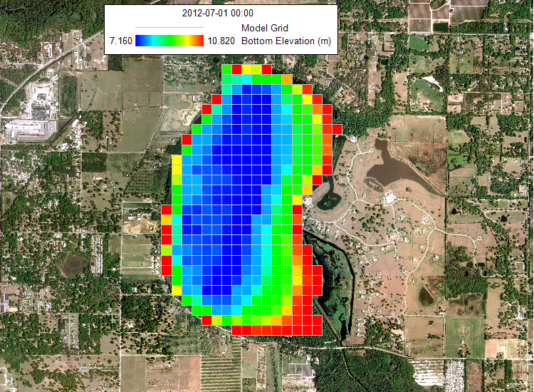
Figure 1. Lake Thonotosassa location map.
2. Description of Hydrodynamic Model
The hydrodynamic model is used as the basis for building a water quality model that is part of this guidance document. Figure 2 provides a representation of the digital terrain model for Lake Thonotosassa. All of the boundary types for the Lake Thonotosassa model are flow boundaries, the locations of flow boundary conditions are presented in Figure 3. Flow discharge and temperature used for the model are shown in Figure 4. Figure 5 shows a wind rose of the wind data.
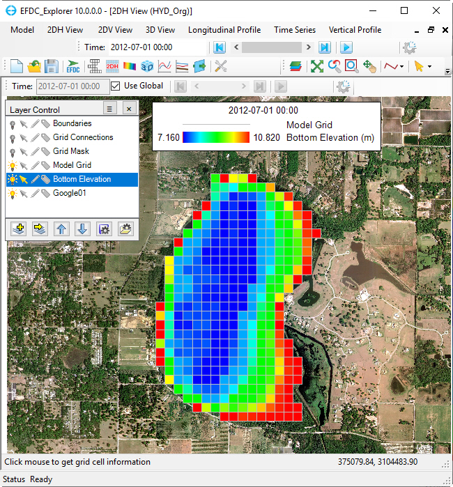
Figure 2. Model bathymetry for Lake Thonotosassa.
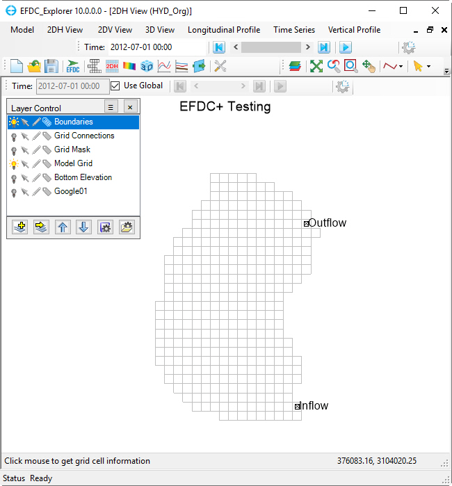
Figure 3. Boundary condition map for Lake Thonotosassa.
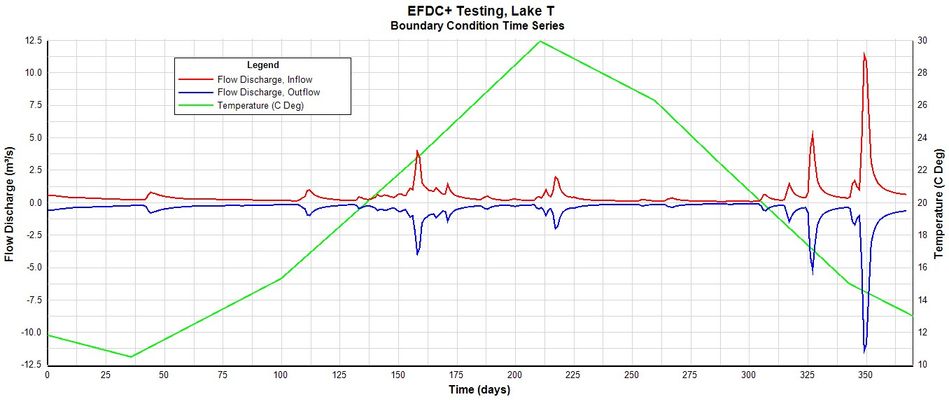
Figure 4. Flow and temperature boundary conditions.
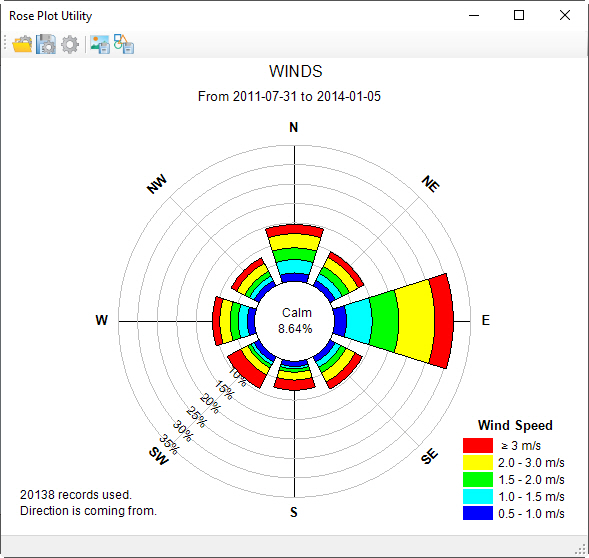
Figure 5 Wind boundary conditions.
3. Setting Water Quality Model
Open the hydrodynamic model then add wind data in the model as shown in Figure 6.
From Model Control form, select External Forcing Data menu item, RMC on Wind sub-option and select Add a Data Series to add wind data series.
Boundary Data Series form is displayed to edit wind boundary.
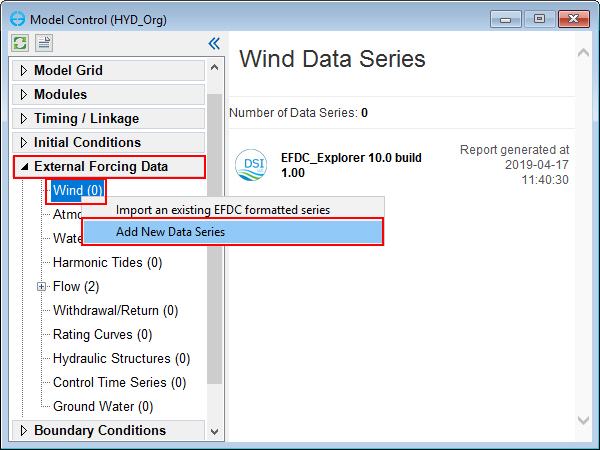
Figure 6. Add new wind data series.
Enter the Number of Series into the # box for adding multiple times series, or click on Add New button to add series one by one. There is one winds boundary so it should be “1” in this case.
Update the Series Name for associated time series. In this case, the title “Winds” for current series 1.
Copy and paste time series data, “Winds.dat,” into the workspace corresponding to the winds as shown in Figure 7 then click the OK button.
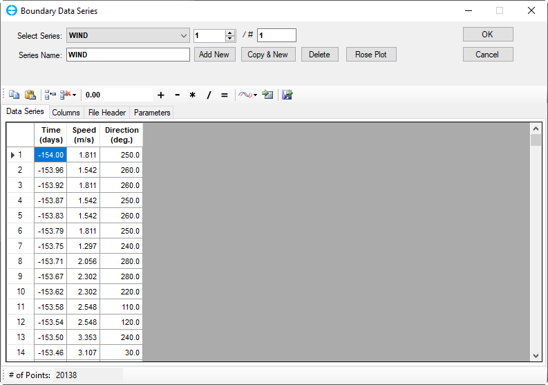
Figure 7. Wind Boundary Data Series form.
From the Model Control form, RMC on Modules the tree menu and check Temperature and Water Quality modules then click OK to activate these modules as shown in Figure 8.
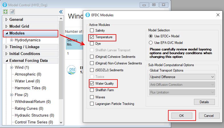
Figure 8 Activate Temperature and Water Quality (1).
After activating Temperature and Water Quality modules, these modules will appear on the left side of the Model Control form, under Modules tree for setting as shown in Figure 9.
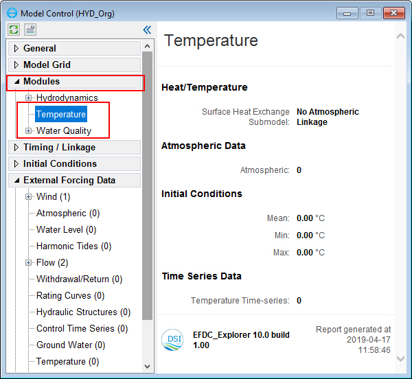
Figure 9 Activate Temperature and Water Quality (2).
3.1 Create the Temperature Boundary Time Series; the Atmospheric Boundary Time Series and set IC for Temperature
1. From Model Control form, RMC on Temperature sub-item, under Modules. Here the user can select (1) Setting to go to Temperature Parameters form to set temperature parameters, (2) Initial Condition to assign temperature IC (Figure 10).
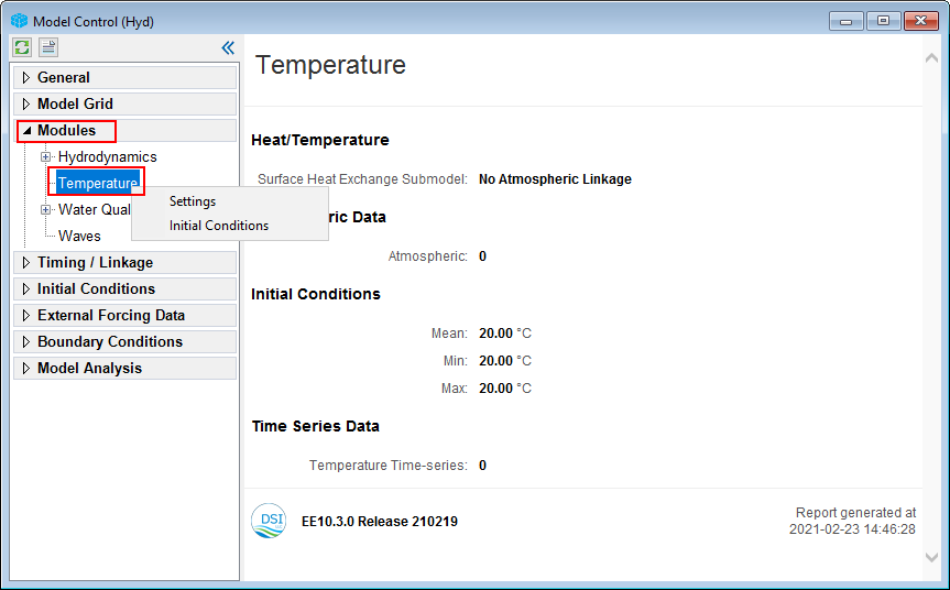
Figure 10. Temperature module setting options.
2. From Model Control form, RMC on Temperature under Modules, select Settings to open Temperature Parameters form as shown in Figure 11.
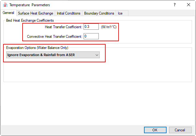
Figure 11. Temperature Parameters form.
2.1. In the General tab, under Bed Heat Exchange Coefficients frame, set Heat Transfer Coefficient value to 0.3, Convective Heat Transfer Coefficient value to 0, as shown Figure 12. The evaporation options can be selected from the drop-down menu,
Figure 12. Temperature Parameters - General setting.
2.2. Move to the Surface Heat Exchange tab, the drop-down list provides several options, including No Atmospheric Linkage, Full Heat Balance, External Equilibrium Temperature, Constant Equilibrium Temperature, Equilibrium temperature (CE-QUAL-W2 method) and Full Heat Balance with Variable Extinction Coeff. Select Equilibrium Temp (CE-QUAL-W2 method) and set parameters as shown in Figure 13.
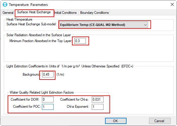
Figure 13. Temperature Parameters - Surface Heat Exchange setting.
2.3. Move to the Initial Conditions tab (shown in Figure 14), set parameters for Bed Temperatures Initial Conditions, then click Assign button in the Initial Conditions for Water Temperature frame to open Apply Cell Properties via Polygons: Temp form to assign temperature IC. Select Use Constant from the Set Initial Conditions and set Operator = 10.5. In the Layer Options frame select Set for All the layers to assign the same value to all layers or select For A Specific Layer to set for each layer, then click on Apply button to assign temperature IC and OK to close the form and return it to the parent form (Figure 15).
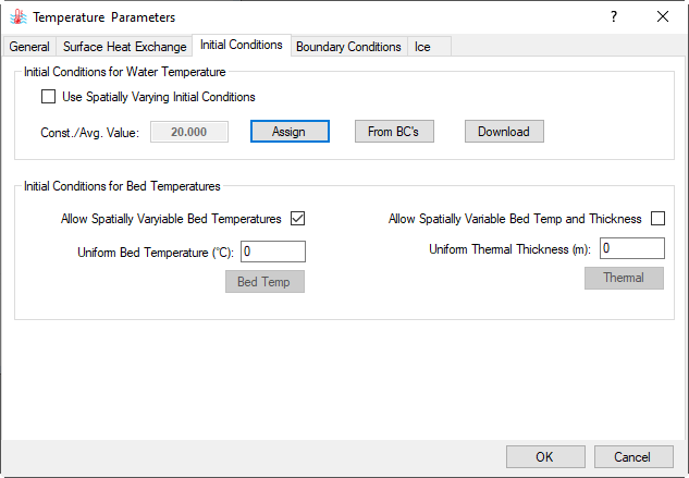
Figure 14. Temperature Parameters - Initial Conditions setting.
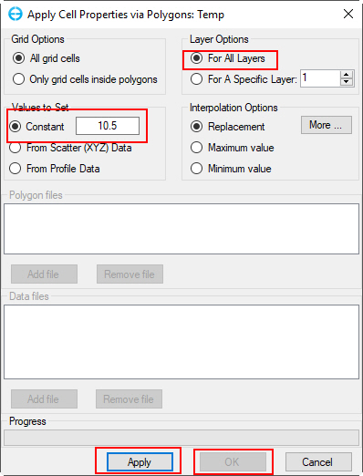
Figure 15. Assign Temperature IC.
2.4. Move to the Boundary Conditions tab. Here the user can create the number of atmospheric and temperature data series as shown in Figure 16.
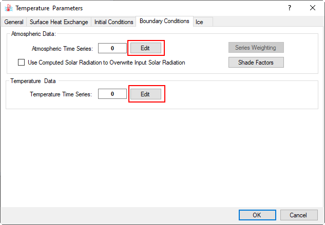
Figure 16. Temperature Parameters - Boundary Conditions setting.
In the Atmospheric Data frame, click on the Edit button then the Boundary Data Series form appears to assign atmospheric data series (Figure 17). Click Add New button to add a new time series then put a name as "Atmospheric" for the Series Name then press Enter key as shown in Figure 17.
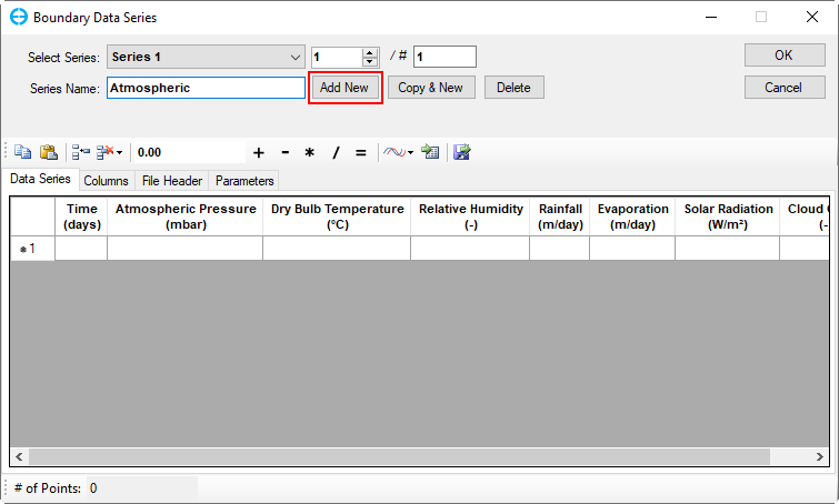
Figure 17. Boundary Condition Settings: Temperature Data Series (1).
Copy and paste time series from “Atmospheric.dat” file from the Data folder, then click OK (Figure 18)
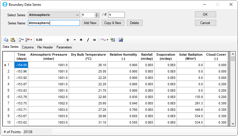
Figure 18. Boundary Condition Settings: Atmospheric Data Series (2).
In the Temperature Data frame (Figure 16), click on Edit button then the Boundary Data Series form appears to assign Temperature data series (Figure 19). Click Add New button to add a new time series then put a name as "Temp Inflow" for the Series Name then press Enter key as shown in Figure 19.
Copy and paste time series from “Temperature.dat” file from the Data folder, then click OK (Figure 20)
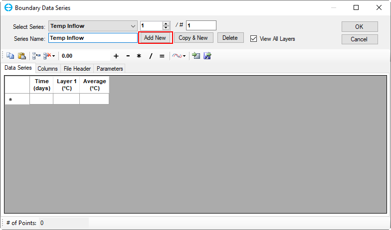
Figure 19. Boundary Condition Settings: Temperature Data Series (1).
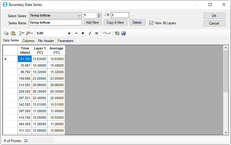
Figure 20. Boundary Condition Settings: Temperature Data Series (2).
3.2 Create the Water Quality Time Series and set Initial Conditions for Water Quality
From the Model Control form, RMC on Water Quality sub-menu under Modules, select Setting to open Water Quality form as shown in Figure 21.
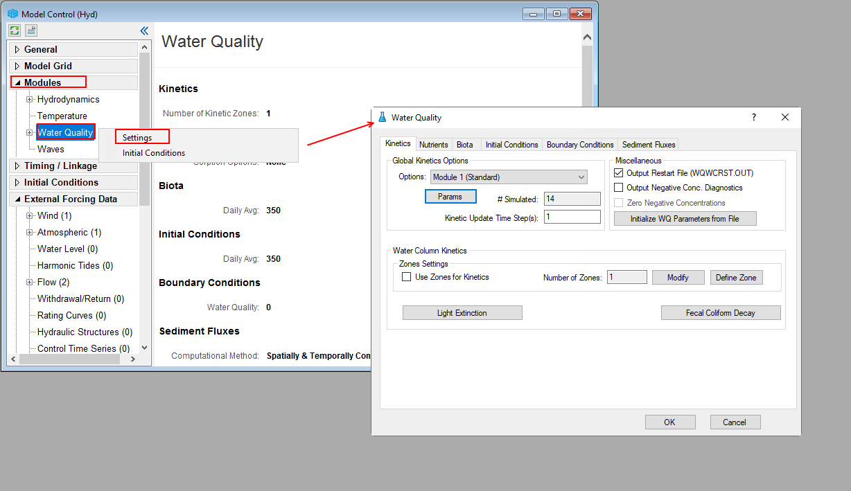
Figure 21. Open Water Quality Settings form.
3.2.1 Water Quality – Kinetics
1. Proceed to the Kinetics tab, select Module 1 (Standard) from the Global Kinetic Options frame dropdown, then click on Params button to display the list of simulated parameters; type 1 for simulated parameter and 0 for not simulated, then click OK as shown in Figure 22.
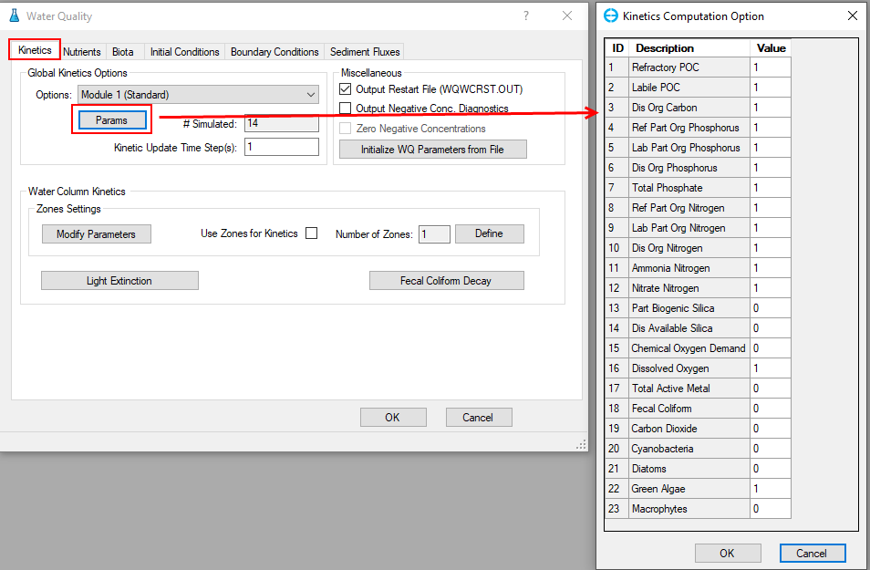
Figure 22. Kinetics Computation Options.
2. Click the Modify Parameter button in Water Column Kinetics frame for Use Zones for Kinetics to edit Kinetic Parameters for the current zone as shown in Figure 23.
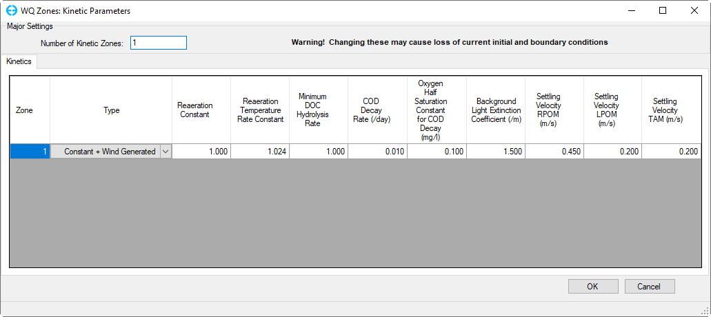
Figure 23. Kinetics Parameters by zone.
3. Click the Fecal Coliform Decay button in the frame Water Column Kinetics to edit Parameter for the current zone as shown in Figure 24.
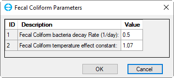
Figure 24. Fecal Coliform Parameters.
4. Click the Light Extinction button in the frame Water Column Kinetics to edit light extinction options as shown in Figure 25.
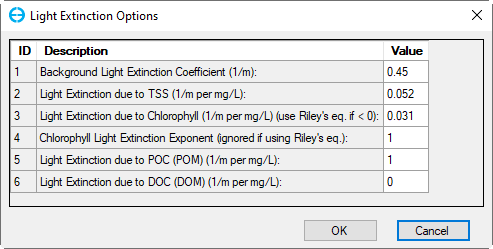
Figure 25. Light Extinction Options.
3.2.2 Water Quality – Nutrients
Proceed to the Nutrients tab as shown in Figure 26.
In the Nutrient Options & Parameters frame: (1) click Temperature Effects button to edit temperature effects as shown in Figure 27; (2) click Carbon button to edit the Carbon parameters as shown in Figure 28; (3) Nitrogen button to edit the Nitrogen parameters as shown in Figure 29; (4) Phosphorus button to edit the Phosphorus parameters as shown in Figure 30; (5) COD&DO button to edit the COD&DO parameters as shown in Figure 31.
In the Sorption Options frame: Select Total Active Metal (TAM) Based option and (6) click Modify Parameters buttons to edit Nutrient Sorption Parameters as shown in Figure 32.
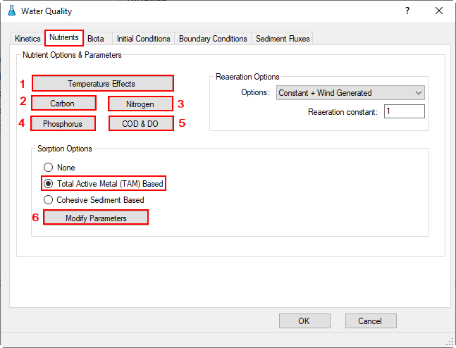
Figure 26. Water Quality Tab: Nutrients.
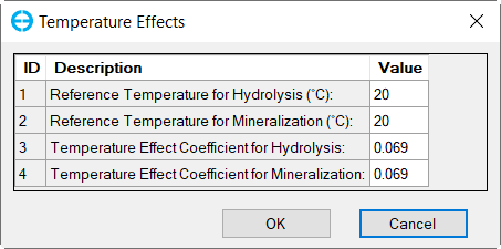
Figure 27. Nutrients: (1) Temperature Effects.
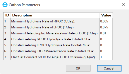
Figure 28. Nutrients: (2) Carbon Parameters.
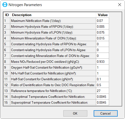
Figure 29. Nutrients: (3) Nitrogen Parameters.
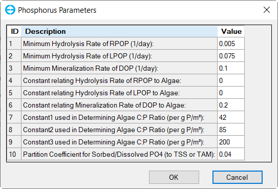
Figure 30. Nutrients: (4) Phosphorus Parameters.
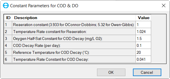
Figure 31. Nutrients: (5) COD and DO Parameters
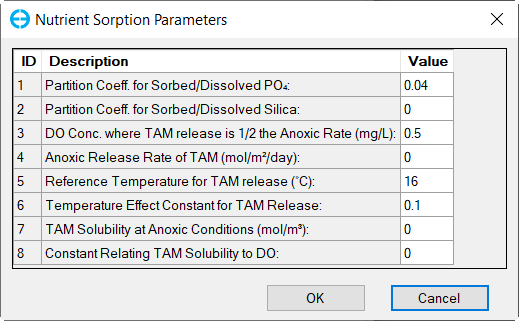
Figure 32. Nutrients: (6) Nutrient Sorption Parameters.
3.2.3 Water Quality – Biota
To configure the algae to the model, proceed to the Biota tab which is shown in Figure 33. By default, there are four algal groups, in this model only one algal group (green algae) is simulated (Figure 22).
In Algae and Macrophyte Options frame: click Modify button, the form of Algae and Macrophyte Options will be appeared as shown inFigure 34. Select Green Algae for Select Biota. Settings for the current green algae through General, Growth, Basal Metabolism, Predation tabs as shown from Figure 34 to Figure 37.
In the Solar Radiation Option for Photosynthesis frame (Figure 33), select source drop-down and select Constant, then click Modify button to edit solar radiation parameters as shown in Figure 38.
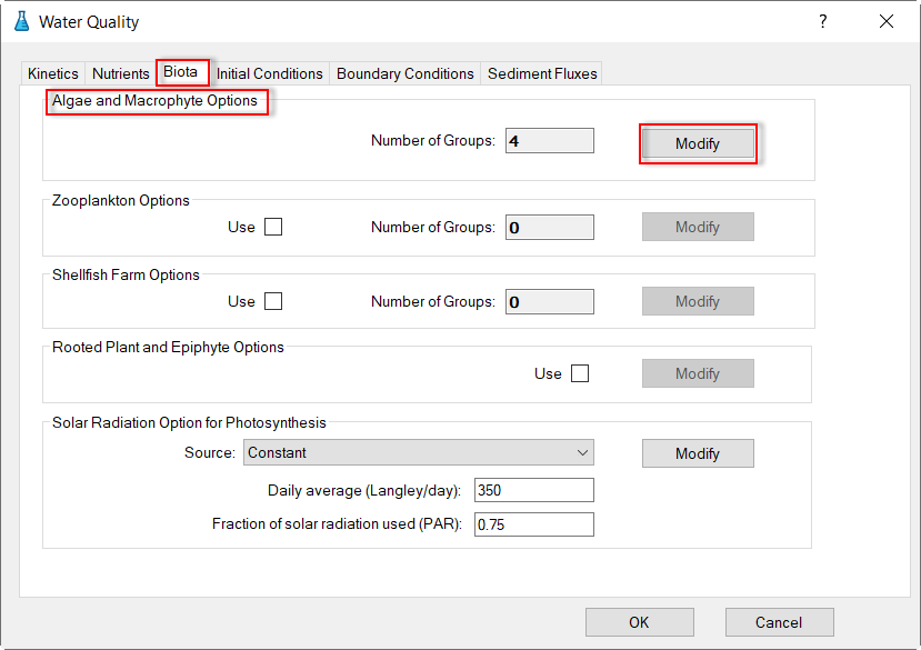
Figure 33. Water Quality: Biota tab.
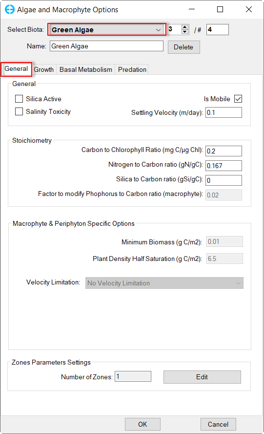
Figure 34. Green Algae: General.
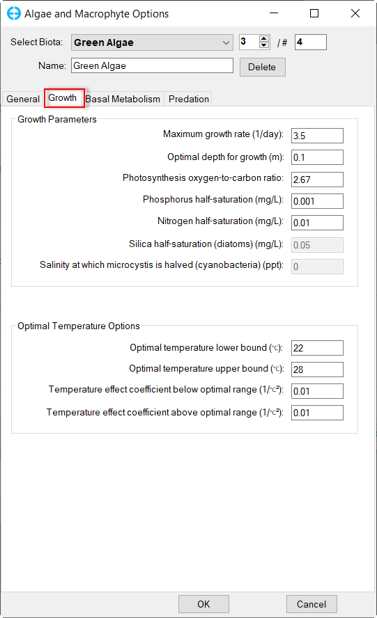
Figure 35. Green Algae: Growth.
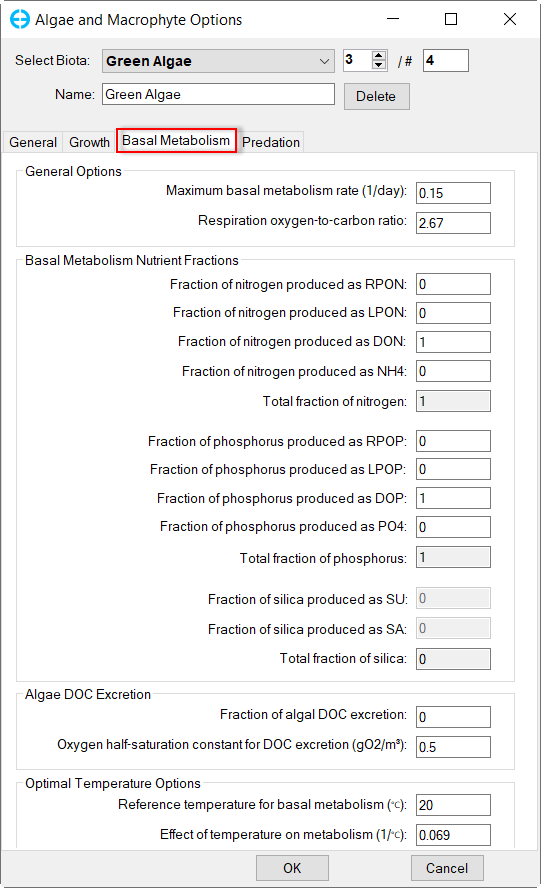
Figure 36. Green Algae: Basal Metabolism.
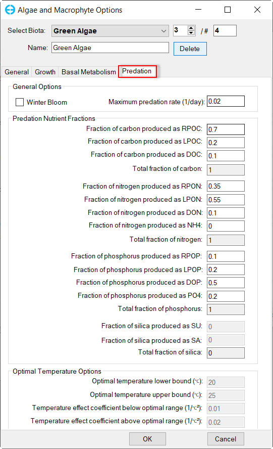
Figure 37. Green Algae: Predation.
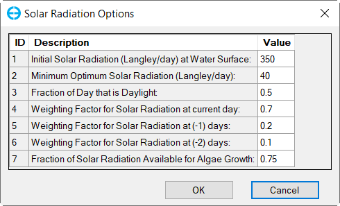
Figure 38. Algae: Solar Radiation Options.
3.2.4 Water Quality – Initial Conditions
Proceed to the Initial Conditions tab as shown in Figure 40. In Initial Conditions frame, click on the drop-down menu and select Spatially Constant, then edit each of the water quality parameters shown in Figure 40 and Figure 41.
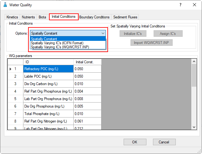
Figure 40. Water Quality Tab: Initial Conditions.
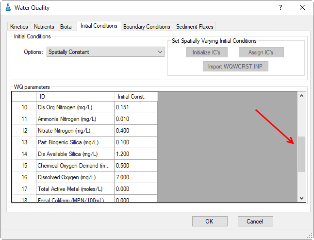
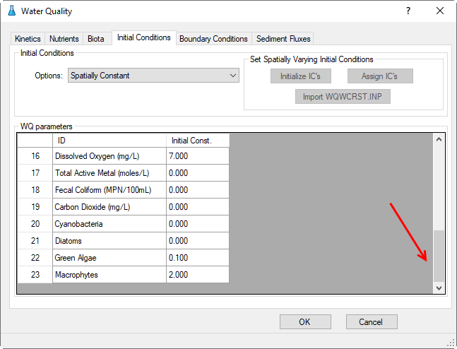
Figure 41. WQ Initial Conditions Parameters.
3.2.5 Water Quality – Boundary Conditions
1. Proceed to the Boundary Conditions tab as shown in Figure 42; Click the Edit button in the Time series Data frame to open Boundary Data Series form which is shown in Figure 43.
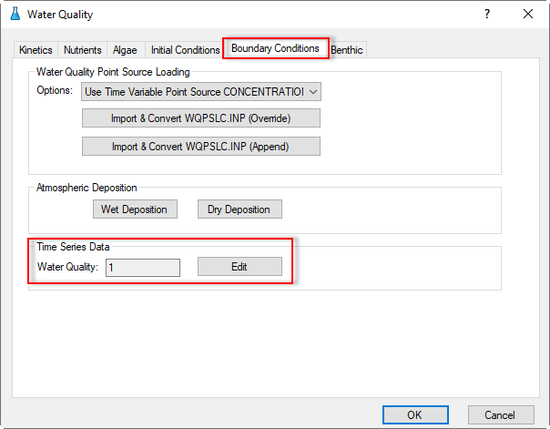
Figure 42. Water Quality Tab: Boundary Conditions.
2. Set the number of series to 1 in # box or click on Add New button to add a data series. Set the Series Name to "WQ Data" and type or copy and paste into the form for the time and cyanobacteria data as shown in Figure 43.
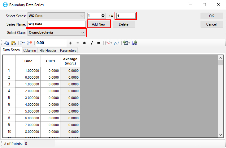
Figure 43. Boundary Condition Settings: Cyanobacteria Data Series.
3. Click on Select Class drop-down menu to select other parameters. Copy and paste into the form for the time and water quality parameter data. An example of the diatom algae parameter is shown in Figure 44.
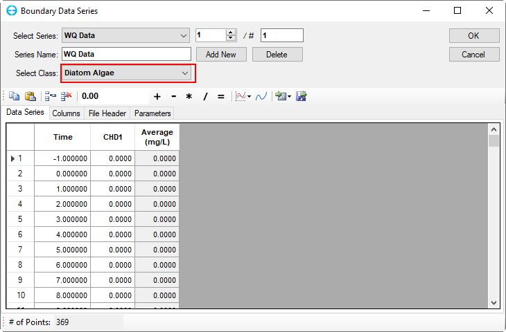
Figure 44. Boundary Condition Settings: Diatom algae Data Series.
5. Repeat this process for the others parameters in the list below:
3) Green algae | Figure 45 | 13) Dissolved organic nitrogen | Figure 55 |
4) Refractory particulate organic carbon | Figure 46 | 14) Ammonia nitrogen | Figure 56 |
5) Labile particulate organic carbon | Figure 47 | 15) Nitrate nitrogen | Figure 57 |
6) Dissolved carbon | Figure 48 | 16) Particulate biogenic silica | Figure 58 |
7) Refractory part. organic phosphorus | Figure 49 | 17) Dissolved available silica | Figure 59 |
8) Labile particulate organic phosphorus | Figure 50 | 18) Chemical oxygen demand | Figure 60 |
9) Dissolved organic phosphorus | Figure 51 | 19) Dissolved oxygen | Figure 61 |
10) Total phosphate | Figure 52 | 20) Total active metal | Figure 62 |
11) Refractory part. Org. nitrogen | Figure 53 | 21) Fecal coliform bacteria | Figure 63 |
12) Labile part. organic nitrogen | Figure 54 |
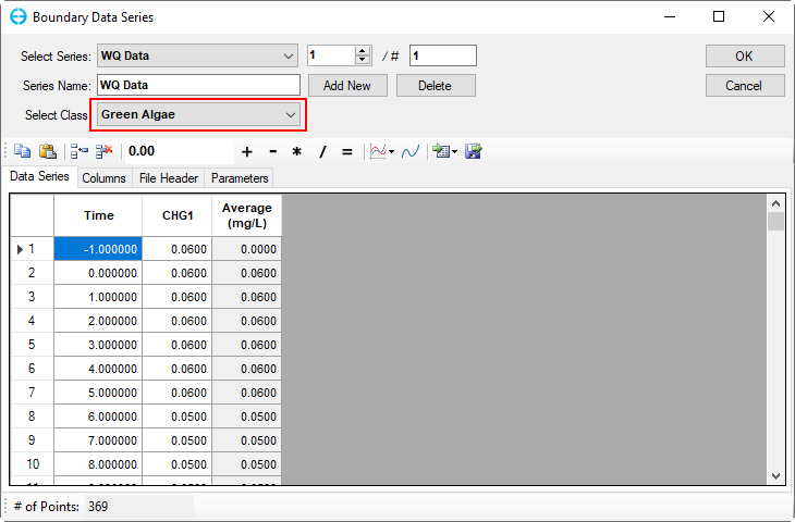
Figure 45. Boundary Condition Settings: green algae.
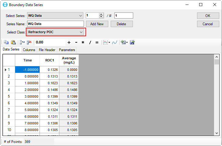
Figure 46. Boundary Condition Settings: Refractory particulate organic carbon.
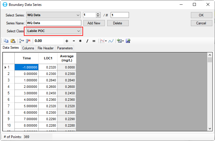
Figure 47. Boundary Condition Settings: Labile particulate organic carbon.
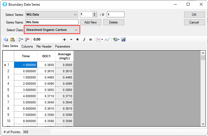
Figure 48. Boundary Condition Settings: DOC.
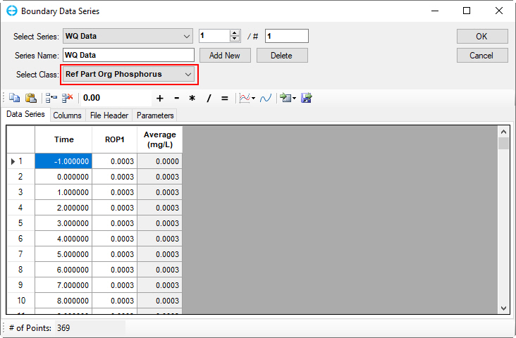
Figure 49. Boundary Condition Settings: Refractory particulate organic phosphorus.
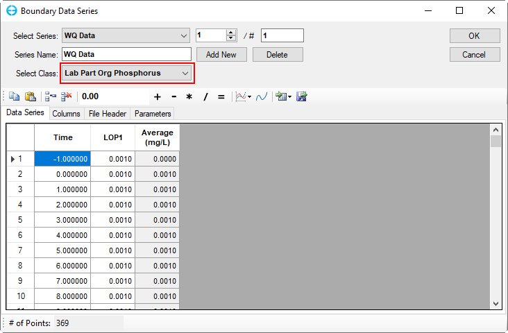
Figure 50. Boundary Condition Settings: Labile particulate organic phosphorus.
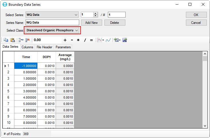
Figure 51. Boundary Condition Settings: Dissolved organic phosphorus.
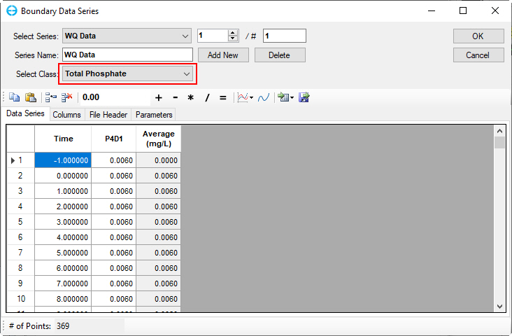
Figure 52. Boundary Condition Settings: Total phosphate.
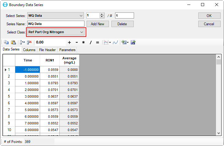
Figure 53. Boundary Condition Settings: Refractory particulate organic nitrogen.
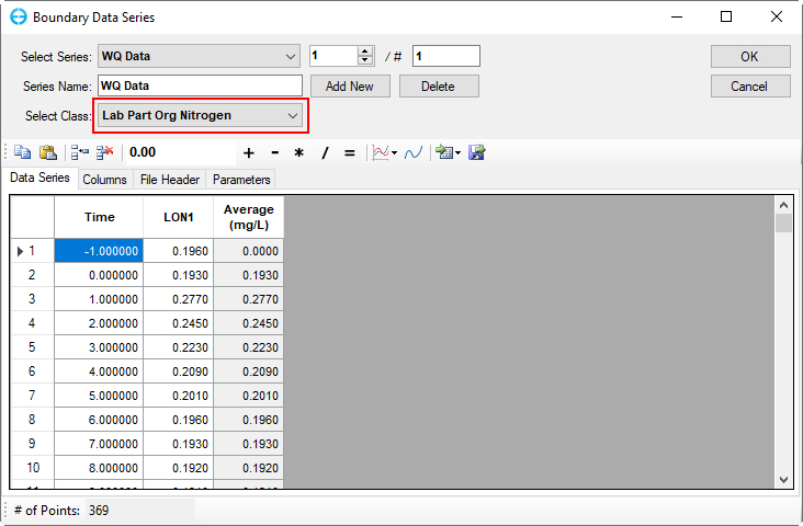
Figure 54. Boundary Condition Settings: Labile particulate organic nitrogen.
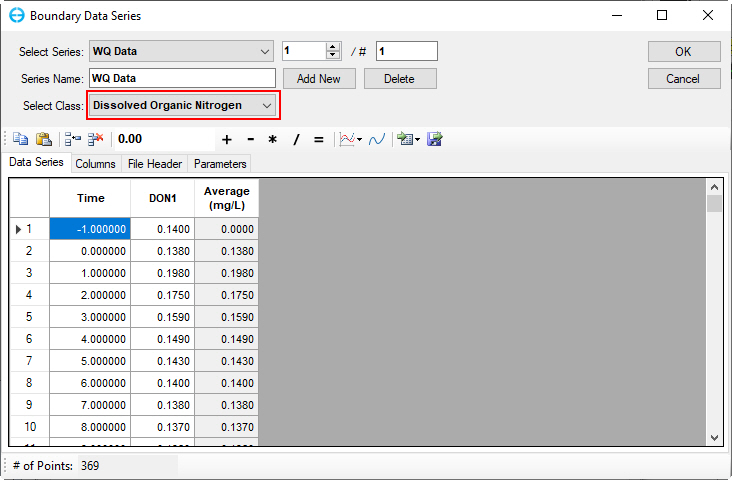
Figure 55. Boundary Condition Settings: Dissolved organic nitrogen.
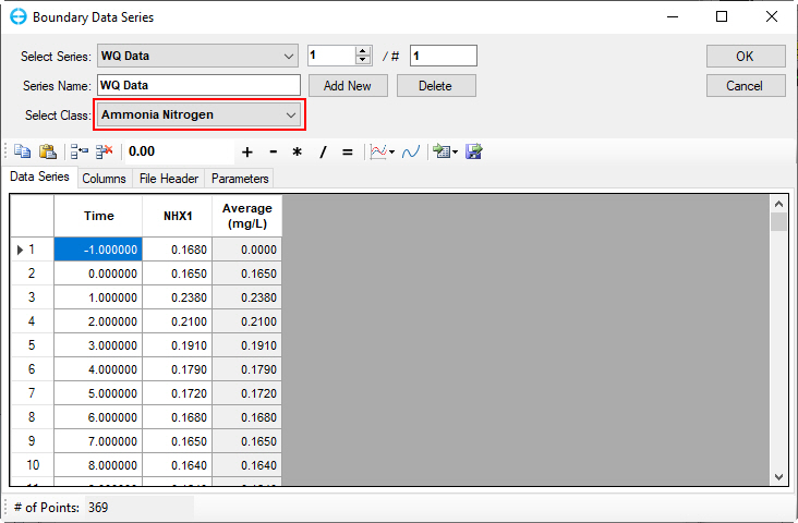
Figure 56. Boundary Condition Settings: Ammonia nitrogen.
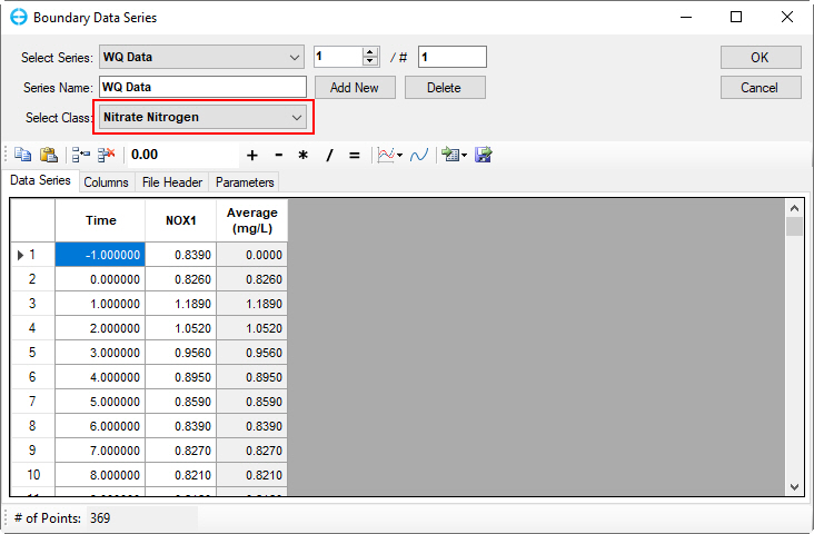
Figure 57. Boundary Condition Settings: Nitrate nitrogen.
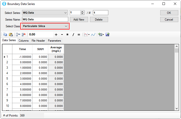
Figure 58. Boundary Condition Settings: Particulate biogenic silica.
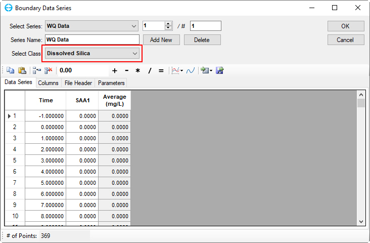
Figure 59. Boundary Condition Settings: Dissolved available silica.
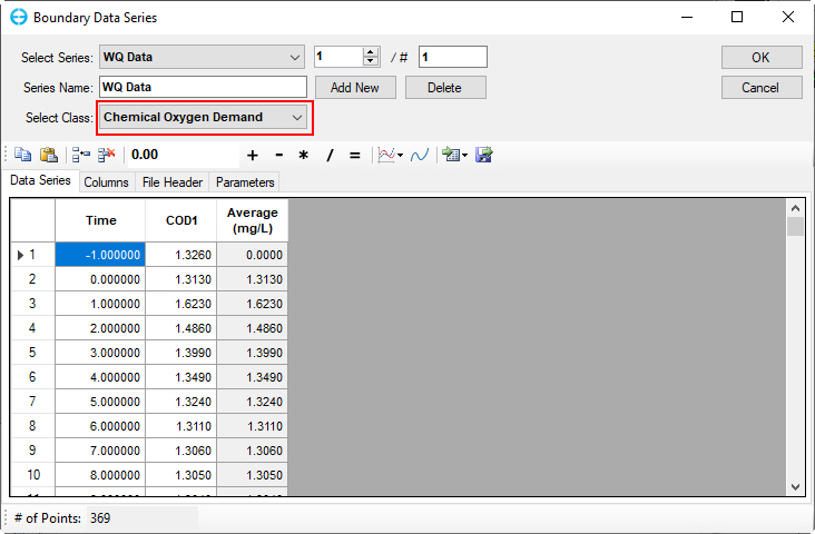
Figure 60. Boundary Condition Settings: Chemical oxygen demand.
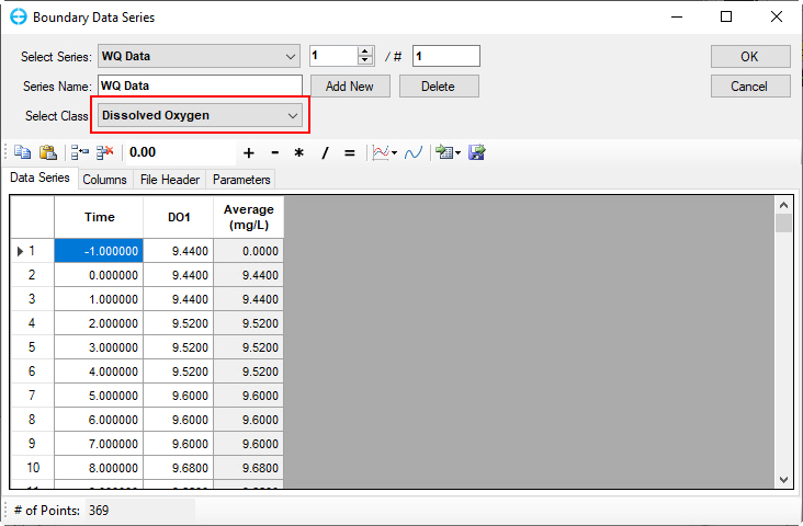
Figure 61. Boundary Condition Settings: Dissolved oxygen.
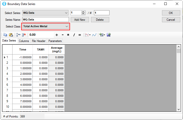
Figure 62. Boundary Condition Settings: Total active metal. 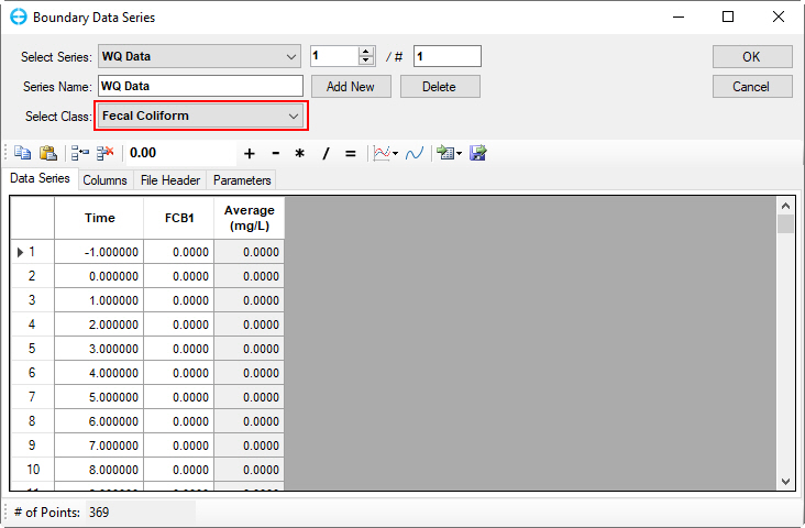
Figure 63. Boundary Condition Settings: Fecal coliform bacteria.
6. Click the OK button when you have finished setting all 21 parameters
3.2.6 Water Quality – Benthic
1. Proceed to the Sediment Fluxes tab shown in Figure 64.
2. Select Modify Parameters button will now displayed under Sediment Fluxes as shown in Figure 65.
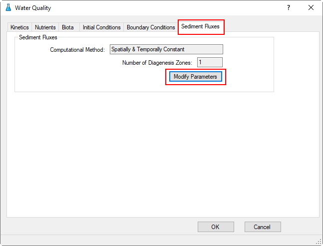
Figure 64. Water Quality Tab: Sediment Fluxes.
3. From the Sediment Diagenesis Option & Parameters form (Figure 65), in the top frame, Benthic Nutrient Flux Method select Spatially & Temporally Constant; enter the values of parameters in the Constant Benthic Flux Rates frame as shown in Figure 65.
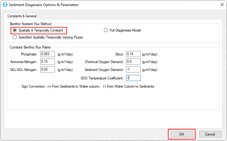
Figure 65. Set Benthic Flux Rates.
4. Click the OK button when finished setting to return to the main form.
3.2.7 Linking the time series to the BC locations
1. From the Model Control form, select Boundary Conditions, expand the Flow boundary group, RMC on Inflow BC group, select Edit Boundary Group (Figure 66) to open Flow Boundary Conditions form (Figure 67)
In the Flow Boundary Conditions form,
2. Set the Time Varying Concentration | Temperature to "Temp Inflow"
3. Set the Time Varying Concentration | Water Quality to "WQ Data"
4. Click E to check which series have been defined if necessary.
5. Click the OK button to save the settings and move back to main form (Figure 67).
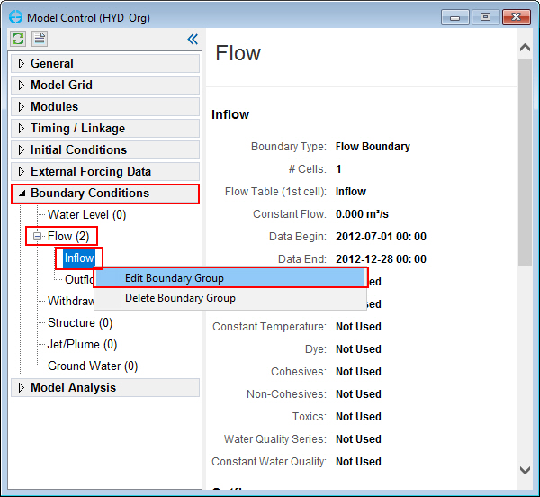
Figure 66. Linking Time series to BC location (1).
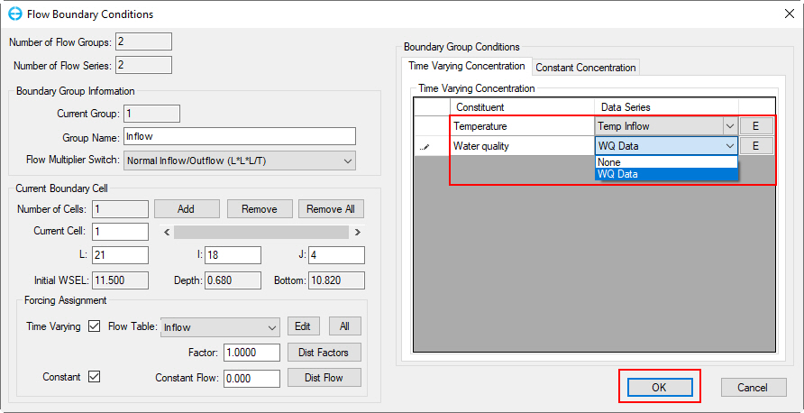
Figure 67. Linking Time series to BC location (2).
6. Click the Save Project button in the main form, the Select Directory: Write Operation will now be displayed. Select Full Write in the Save Options frame; click OK as shown in Figure 68.
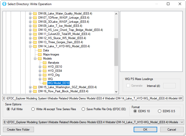
Figure 68. Apply Full write of the model.
4. Running the Model
1. From Model Control form, select the Timing/Linkage menu item and RMC on Timing sub-option
2. Set the Model Start Time to 182;
3. Set # of Reference Periods to 180;
4. Set Duration of Reference Periods to 24;
5. Set Time Step to 10, then click the OK button to save setting as shown in Figure 69.
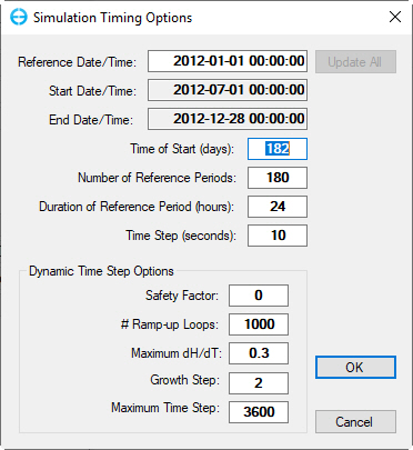
Figure 69. Model Control Form – Timing/Linkage: Timing.
6. RMC on Linkage sub-option to open EFDC Model Linkages form, in the EFDC+ Explorer Linkage frame, set the Linkage Output Frequency under EFDC+ Explorer Linkage frame to 60 minutes as shown in Figure 70.
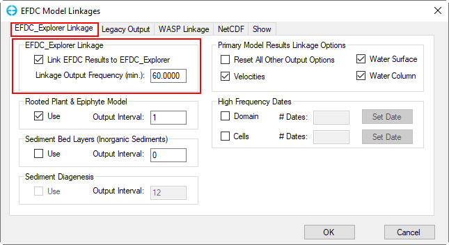
Figure 70. Main Form – Timing / Linkage: EFDC+ Explorer Linkage.
7. Click the Run EDFC  icon on the toolbar to open EFDC+ Run Options form; in the General tab, enter the number of OMP Threads, KMP Offset and check the executable file then click Run EFDC+ button to run the model as shown in Figure 71.
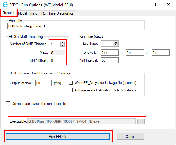
Figure 71 EFDC+ Run Options form.
5. Viewing Water Quality in EFDC+ Explorer
1. 2DH View
1. After the model run has finished, from the toolbar, click on icon or select 2DH View\ New 2DH View from the toolbar to open the 2DH View window as in Figure 72 below.
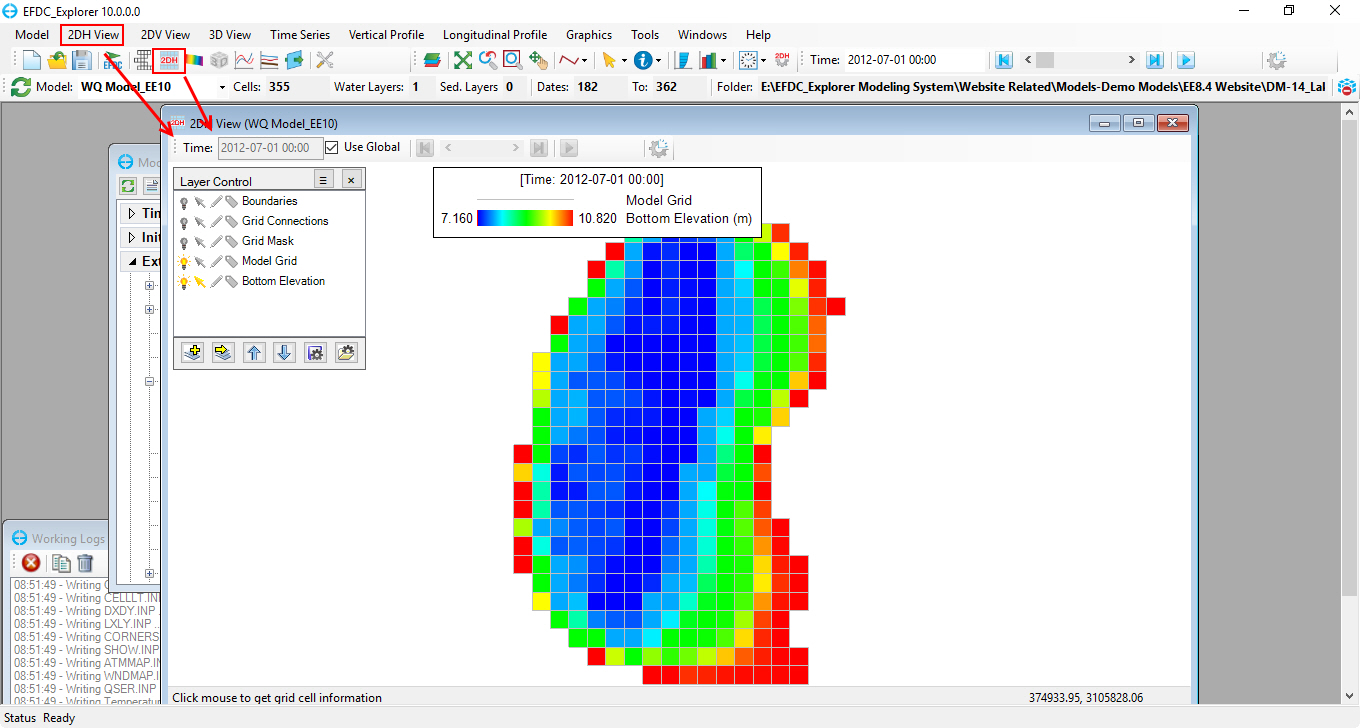
Figure 72. 2DH View window.
2. From 2DH View window, select  icon on the lower left corner of Layer Control frame or RMC in the blank area of the Layer Control frame and select Add New Layer (Figure 73).
3. The View Option form appears to add layer into 2DH View. From the View Options form, (1) click on drop-down menu and select Water Quality group under Primary Group; (2) select parameter that the user want to view; (3) select view layer settings; then click Add button to add new layer into 2DH View window (Figure 73).
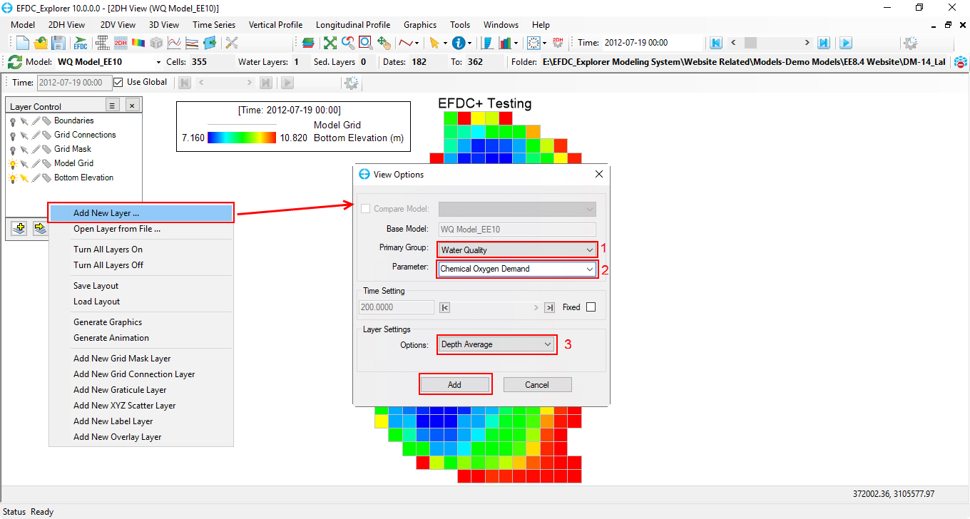
Figure 73. Add New Layer into 2DH View window.
2. 2DV View (ViewSlice Mode)
1. From the main form, click on  button or select 2DV View\ New 2DV View on the toolbar to open the Data Extraction for Vertical Profile Slice Plots form as shown in Figure 74
2. From Data Extraction for Vertical Profile Slice Plots form,
2.1 (1) Profile Definition option: user can select view profile as a grid column (I direction), grid row (J direction) or based on a polyline (Use Drape File).
Note: Users should remember to browse to a polyline used to extract vertical slice when selecting Profile Definition as Use Drape file
2.2 (2) Select modules and parameters used to plot vertical slice
2.3 (3) Load/Save setting or delete parameters that the user doesn't want to plot
2.4 Click OK button after selecting all options above to close the form and plot the vertical slice.
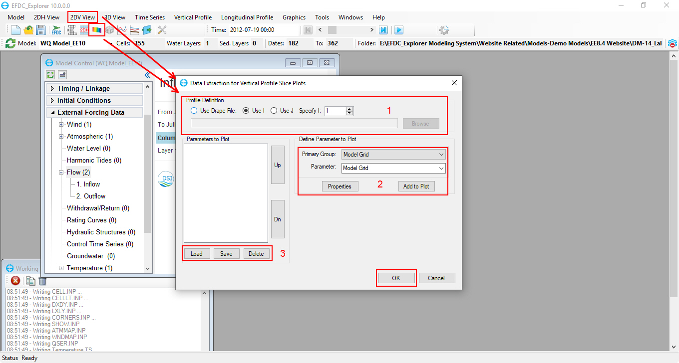
Figure 74. Data extraction for 2DV plots.
The user can define a polyline by clicking Draw a Polyline on 2DH View window to draw a polyline then RMC to end; After drawing the polyline, RMC on Overlay layer in Layer Control frame and select Properties to set the polyline properties or Save As to save the polyline that can later used for slice/extraction as shown in Figure 75.
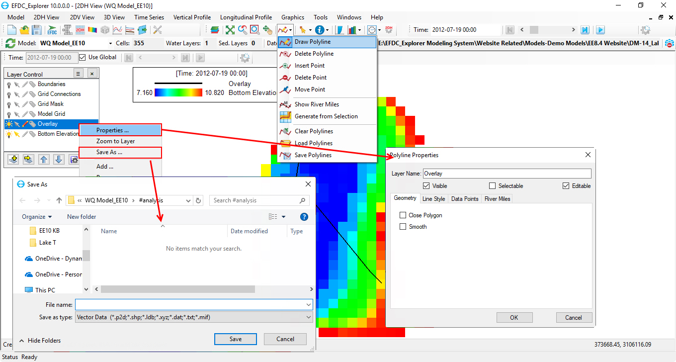
Figure 75. User defined 2DV extraction line definition.
From the 2DV View window, RMC on the Legend and select (1) Properties to set 2DV View properties; or (2) Edit to modify parameters used to plot in the 2DV View window (Figure 76).
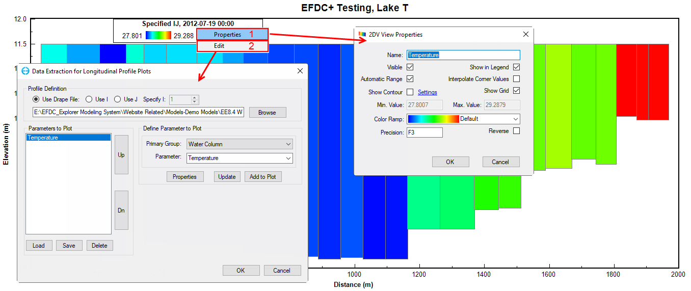
Figure 76. 2DV View window.
3. Longitudinal Profile Plot Mode
1. From the main form, click on  icon or select Longitudinal Profile\ New Longitudinal Profile on the toolbar to open Data Extraction for Longitudinal Profile Plots form as shown in Figure 77.
2. From the Data Extraction for Longitudinal Profile Plots form, set the same setting steps as 2DV View Plots in Figure 74 earlier.
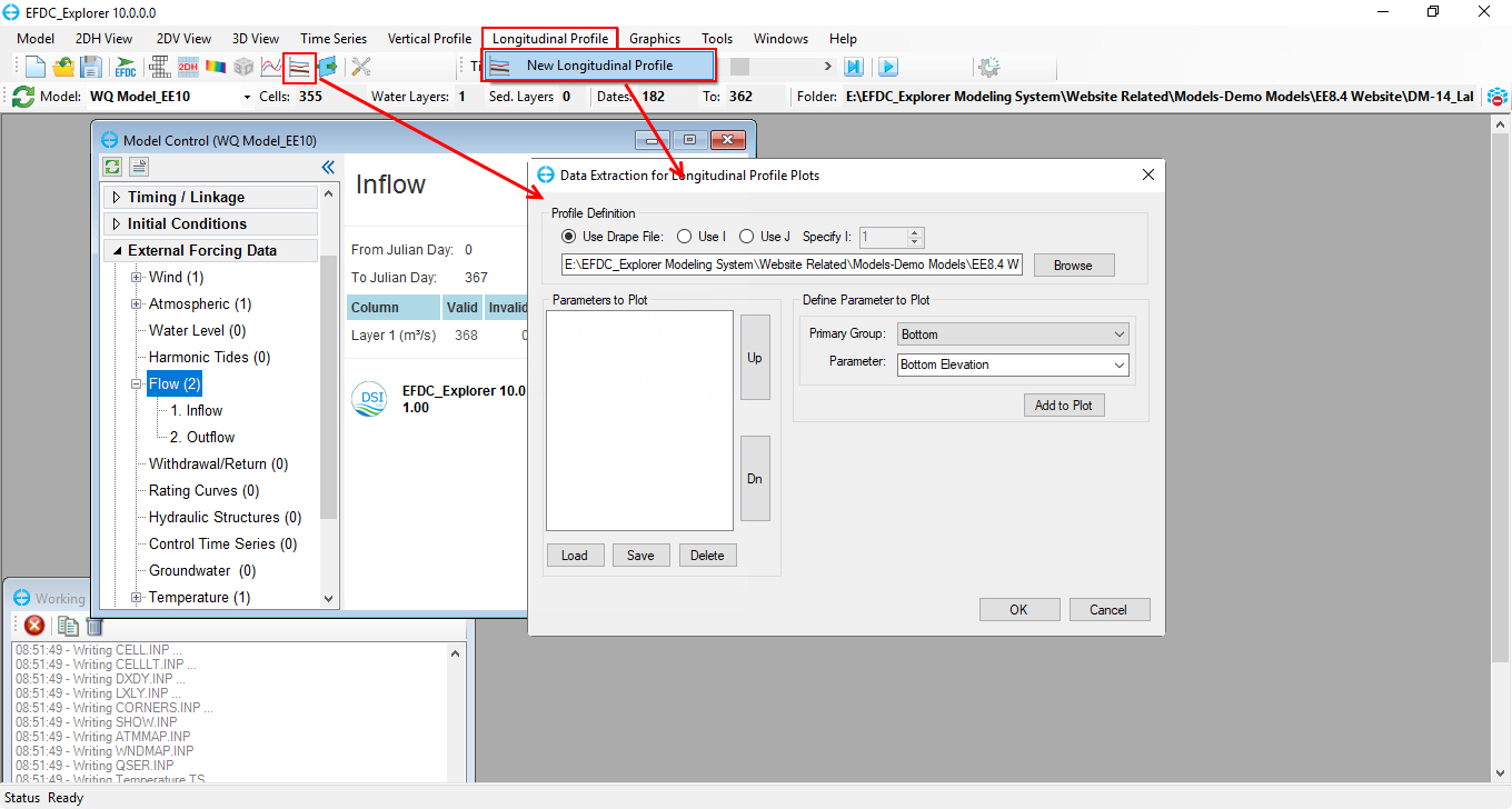
Figure 77. Data Extraction for Longitudinal Profile Plots form.
3. From the Longitudinal Profile Plot window, the user can customize plots, save plot settings, generate plots as an EMF file or an animation. The user can export data to an ASCII file or import other data into this window by using the options in the icons from the toolbars.
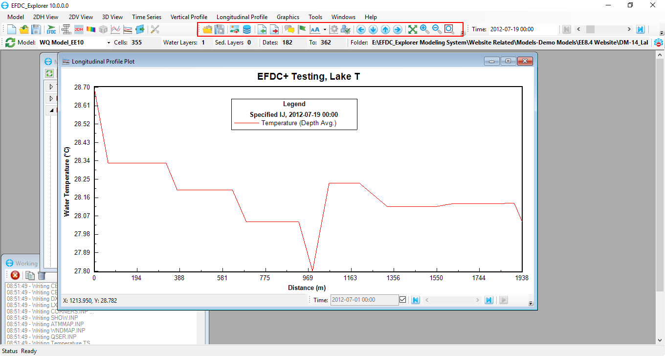
Figure 78. Longitudinal Profile Plot window.
End