1. Introduction

The model is set up to replicate the Pasche and Rouvé (1985) test cases for vegetation interactions in the flume described in the paper “3D numerical modeling of open-channel flow with submerged vegetation”. The goal of the project is to understand better the impact of vegetation on the flow in an open channel.

All files for this tutorial are contained in the Test Case of the Resources page folder file (TC-11_Rigid Vegetation_Test_Case).

The experiments are considered to verify the model's capability in accurately simulating shallow flow hydrodynamics in the presence of vegetation. The experiment was carried out in a 25.5 m x 1.0 m compound channel with a floodplain covered by vegetation. The cross-section of the channel is shown in Figure 1 below.

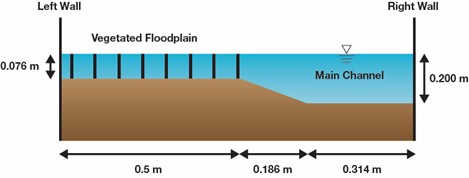
Figure 1.  Cross-section of the channel.

2. Data Summary

2.1 Cross-section

Based on the experiment cross-section, three polygon files have been prepared, for the floodplain, slope, and main channel; the dimensions of these polygons are summarized in Table 1.

Table 1: Cross-section polygon dimensions

2.2 Water depth/Surface Elevation

Water depth refers to the measurement of the surface elevation of rivers, lakes, oceans, seas, or other large bodies of water, and is of primary importance for hydrodynamic modeling.  Data used for generating the initial conditions measurements of water depth are available as a text file with three columns (Figure 2).  The first line is a comment line, marked by an asterisk.  Each subsequent line has coordinates (X and Y) and the value of the elevation.  These data files can be converted from other data sources such as DEM data or topo maps, which can be surveyed or downloaded from the internet. The raw water depth data used for this model are shown in Figure 2.

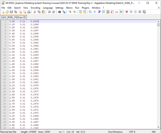
Figure 2. The raw data format used for generating water depth initial conditions in the model

2.3 Data Summary 

An overall summary of the data files contained in the Data folder is shown in Table 2.

Table 2.  Data summary 

Note: A polyline or polygon file (*.p2d) is a specific file type commonly used in EE and other tools developed by DSI.  Using three columns in an X, Y, Z tab-delimited format, any number of polylines/polygons can reside in the same file. Users should refer to Appendix B, Data format B-1 of the EE Knowledge Base for more information on this format.

3. Step-by-Step Guide for Building a Model

3.1 Generate a New Model

In this section, we will generate a new hydrodynamic model of the Pasche Test Case.  This exercise will familiarize users with the basic interface of EE and demonstrate how to build a model from scratch.  To load the model interface, double-click on the EEMS icon on your Desktop or start it from the list of programs.  Click on the New Model button to begin generating a new model, as shown in Figure 3.

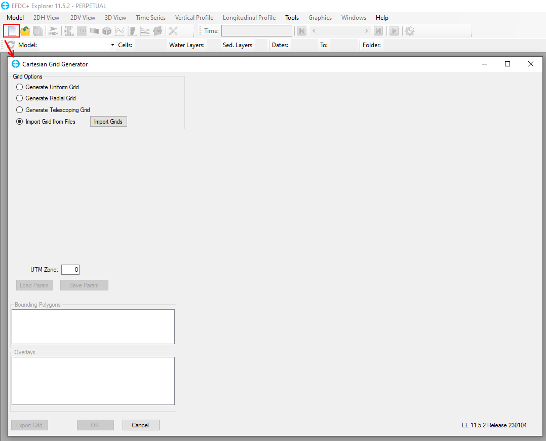
Figure 3. EE main form.

For this exercise, we will generate a Cartesian grid using the following steps.  From the Cartesian Grid Generator form (refer to the step numbering in Figure 3‑3):

1. Select Generate Uniform Grid from the Grid Options frame;
2. Set the dimensions of the uniform grid as shown in Figure 3;
3. In the example, leave the UTM Zone as 0;
4. After filling in the parameters, click the Generate button to generate the model grid, then click on the Remove Dry button to remove cells outside the polygon.  The preview of the generated grid will show in the right panel. 

Note: If the grid is not suitable for your purpose, you can modify the grid parameters and click Generate again to re-generate the grid;

5. After the grid is generated, click the OK button to close the form and go to model settings. In general, clicking OK in all forms will close the form, save settings, and return to the Model Control form.   

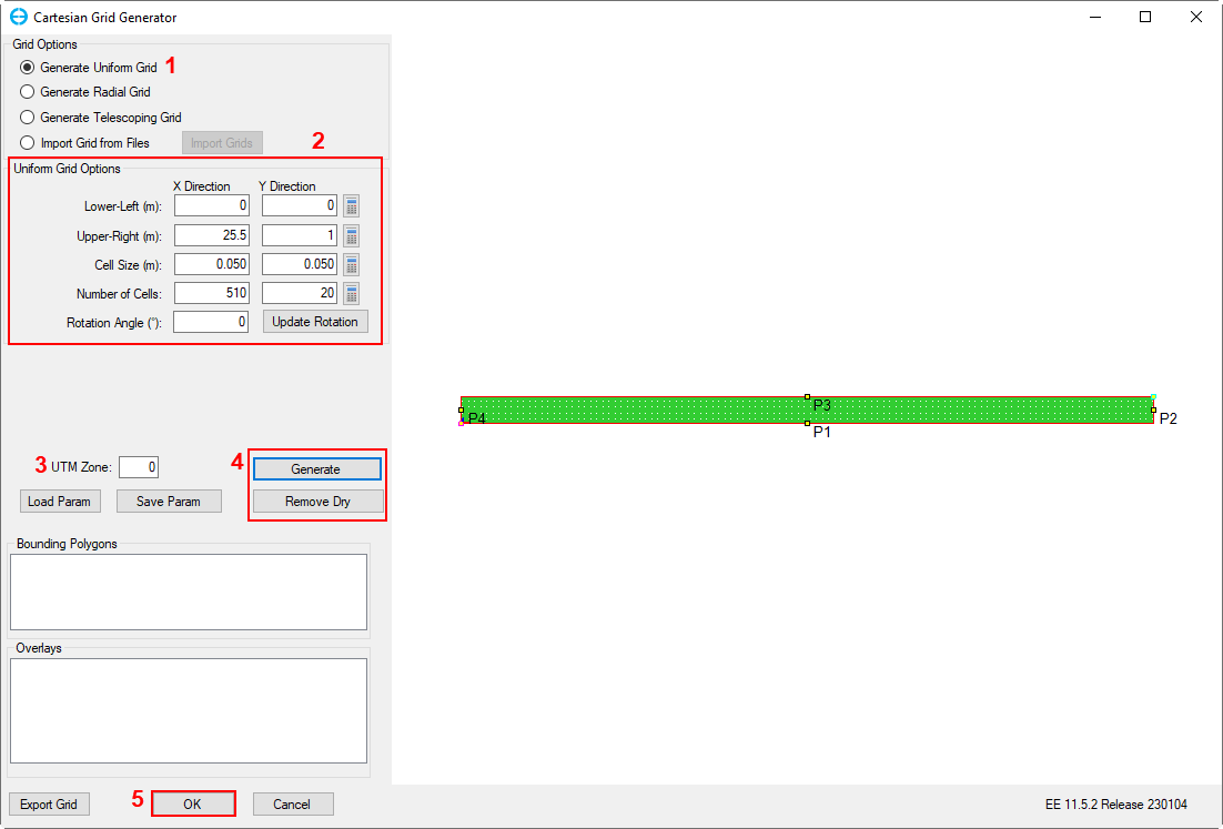
Figure 4.  Generate an EFDC model from scratch.

After the grid is generated, the Model Control form will be displayed in Figure 5.  General information about the model will be displayed that includes the model title, area, number of cells, model width, height, and model location coordinates. 

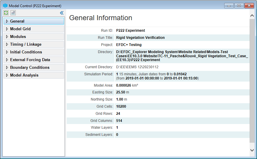
Figure 5.  EE Model control form.

In the model interface, click on Save to save the model, as shown in Figure 6, below

Figure 6. Save Button in the Model Interface

After clicking on the Save button, a Select Directory: Write Operation pop-up will appear to select saving options (refer to Figure 3‑5).  Before project files are saved, the grey box is empty.  This is where EE project files will be listed.  The empty gray box shows that no files have been written yet for the study, as shown in Figure 7. 

Three save options are offered in the Save Options frame of Figure 7:

• Full Write can be selected to save all the input files,
• Write All except Time Series Files can be selected to save all input files without the time series.
• Save Profile File Only (EFDC.EE) can be selected for saving if the user has only changed formatting options in EE.

In this project, the Full Write option is recommended. After choosing this option, click OK to close the form and save the model.

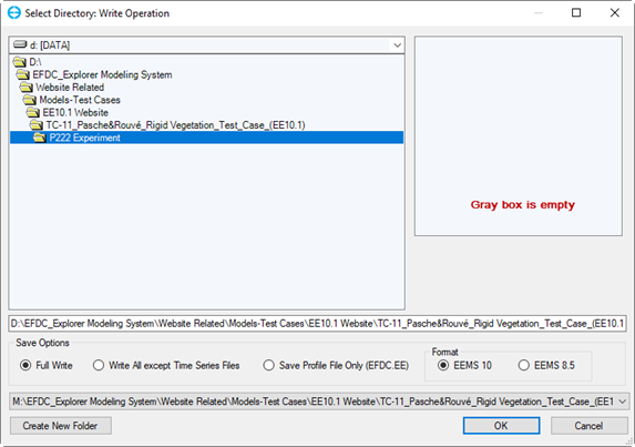
Figure 7. Saving the model.

3.2 Assign Model Bathymetry

The next step in the model setup is to assign the bathymetry for the model domain.  Assigning bathymetry refers to assigning an elevation value to each cell in the model.

You can also click on the 2DH View button which provides access to the utility for viewing two-dimensional (2D) plan views of the model.

Figure 8. 2DH View button in the model interface.

First, click the 2DH View button, which will cause the 2DH View form to appear, then follow the steps below to set the bathymetry (IJ slope) for the floodplain, as shown in Figure 9:       

1. Activate the model editing for the bottom elevation layer by clicking Bottom Elevation in the Layer Control form on the left side of the 2DH View form.
2. In the Selection Tool, select Inside Polygons in File.
3. From the Open Polygon File form that pops up, select the file named floodplain_Plg.p2d.

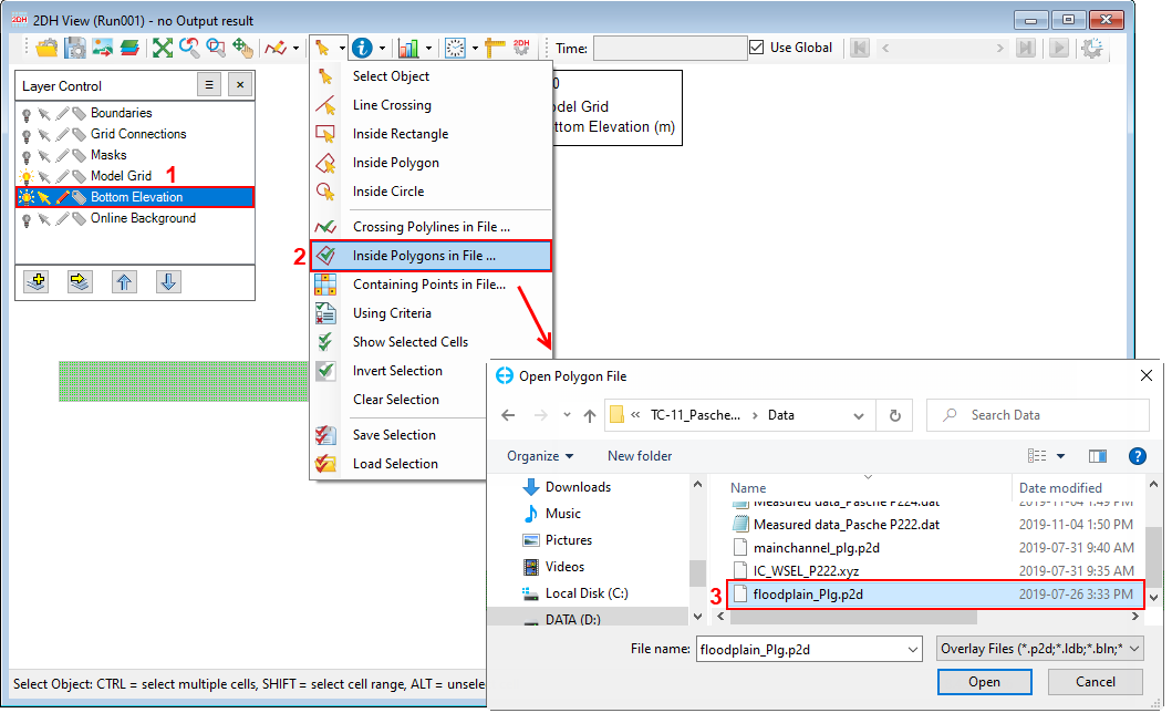
Figure 9.  Set IJ slope for the floodplain.

4. Click the Grid Cell Tool and assign the floodplain slope along the I and J cell indices by selecting Set IJ Slopes, as shown in Figure 10.

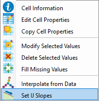
Figure 10.  Grid cell tool.

Selecting Set IJ Slopes applies a constant bed slope to the cells in the I direction or J direction or both IJ directions. Start with a specified initial bottom elevation by putting a value to Start Value then enter a value for I Slope and J Slope. If the entered slope is positive, the bottom elevations will decrease with higher I's and J's. The inverse is true if the entered slope is negative.

For more information on Set IJ Slopes, please refer to the EFDC+ Explorer Knowledge Base: Set IJ SLopes

5. For the floodplain, the bed slope is assigned using the values shown in the Assign Slope pop-up form in Figure 11.

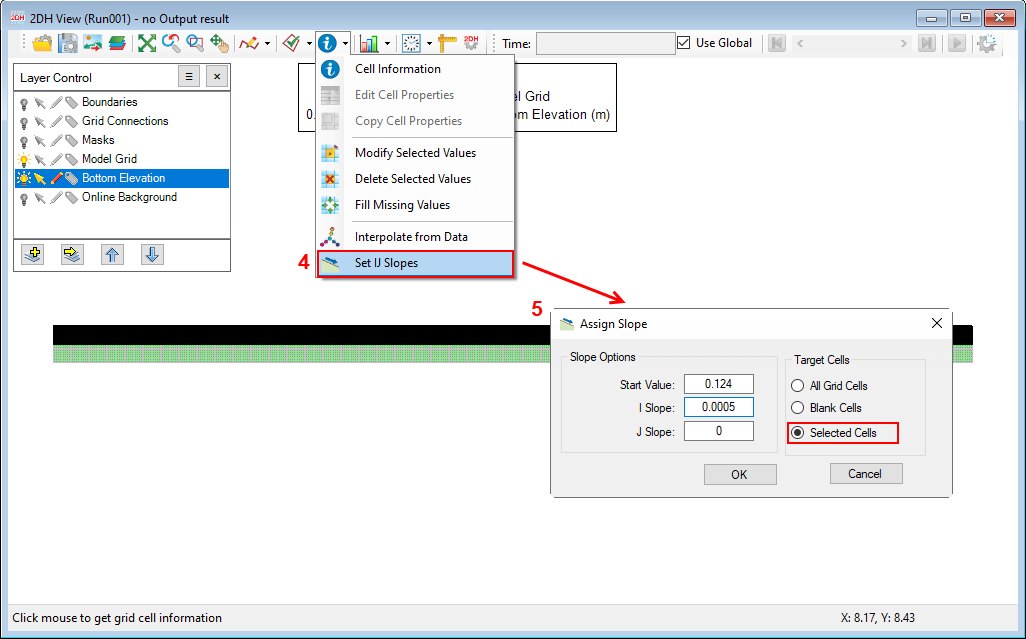
Figure 11. Set IJ slope for the flood plain cross-section.

Take similar steps to assign the bed slope for the slope area and the main channel area. 

For the slope area, follow the instructions associated with Figure 8, Figure 9, and Figure 10, but when the Open Polygon File form appears, select the file named slope_plg.p2d.  Then assign the bed slope with the IJ slope values shown in Figure 12.

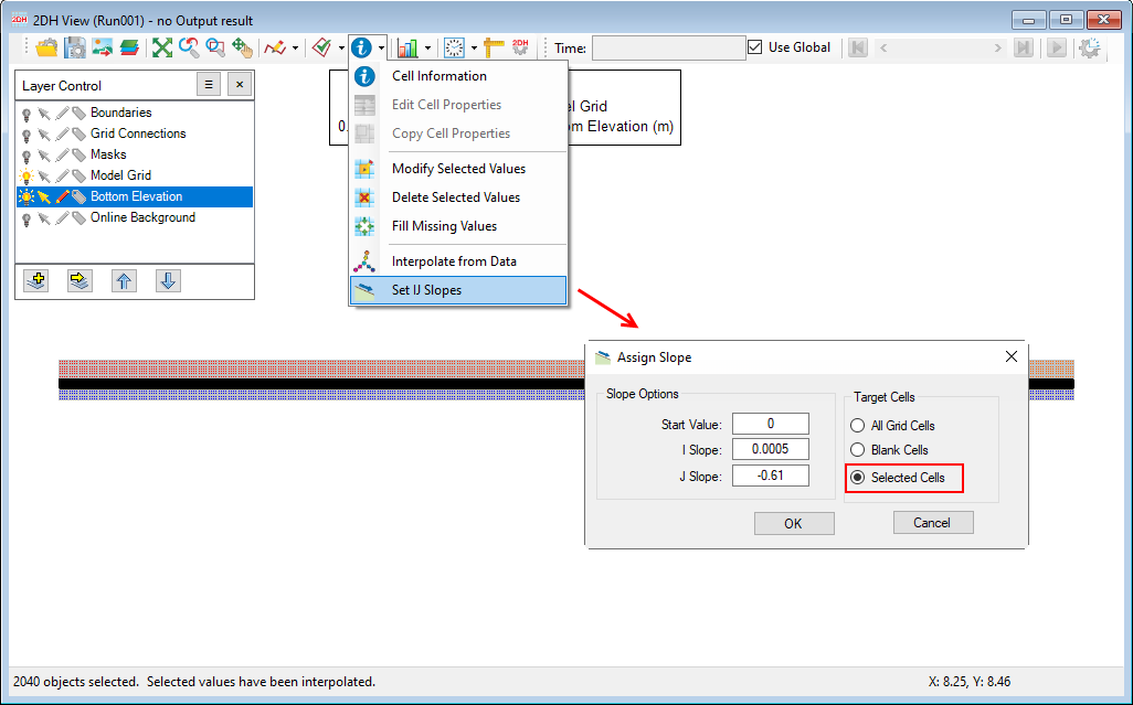
Figure 12.  Set IJ slope for the slope cross-section.

For the main channel, follow the instructions associated with Figure 8, Figure 9, and Figure 10, but when the Open Polygon File form appears, select the file named mainchannel_plg.p2d.  Then assign the bed slope with the IJ slope values shown in Figure 13.

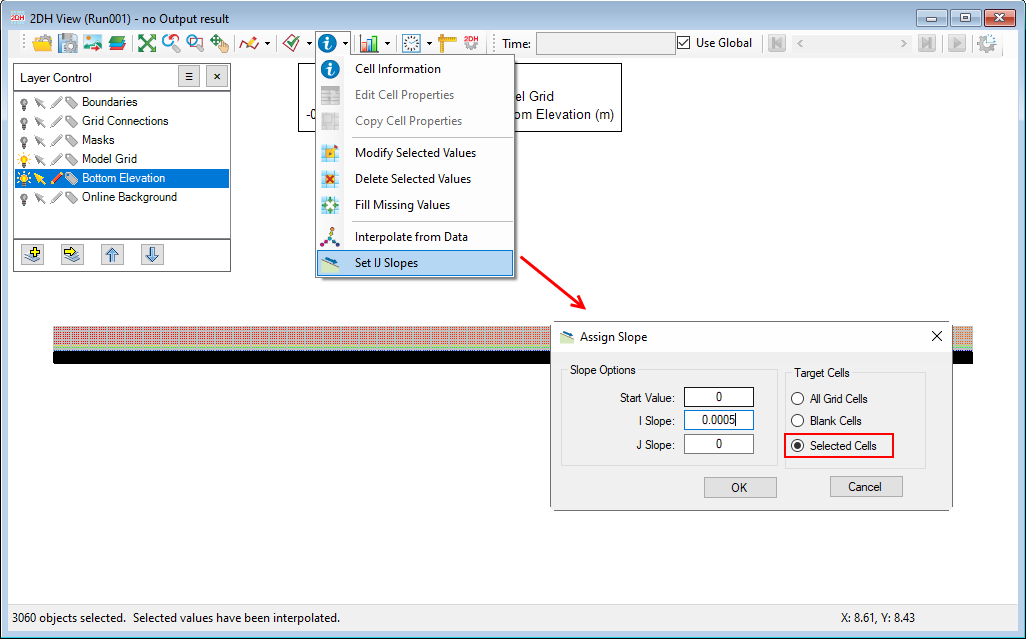
Figure 13.  Set IJ slope for the main channel.

After assigning the model bathymetry, statistical information for the model bathymetry will be reported in the bathymetry report in the right-side panel of the Model Control form as shown in Figure 14. 

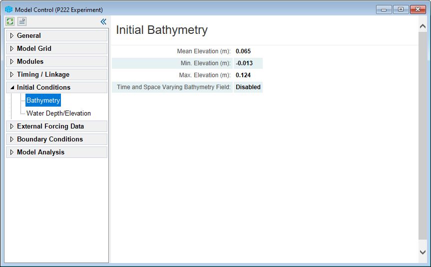
Figure 14.  Statistical information of the model bathymetry.

Figure 15 presents the bottom elevation of each grid cell in the model domain.

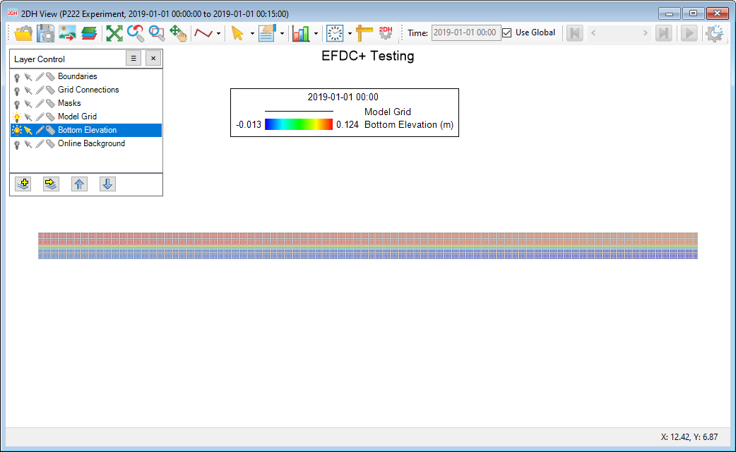
Figure 15.  2DH View form showing model bathymetry.

3.3 Assign Water Surface Elevation

Water surface elevation can be assigned following the import of bathymetry. 

In the Model Control form, as shown in Figure 16:

1. Expand the Initial Conditions tab on the left-hand side
2. RMC on Water Depth/Elevation
3. The Water Depth/Surface Elevation form will appear; click on the Assign Elevation button to assign model water depth.

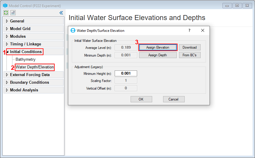
Figure 16.  Assign initial water surface elevations and depths.

After clicking on Assign, the Apply Cell Properties via Polygons: Water Surface Elevations form will appear, which is shown in Figure 17.  In this form:

1. In the Values to Set frame, select Scatter (XYZ) data
2. In the Data Files frame, click on the Add File button to browse to the water surface elevation data file named “IC_WSEL_P222”,
3. Click on Apply Defined Conditions to assign the model water elevation.  This sets the water elevation data from the IC_WSEL_P222 file to the model.

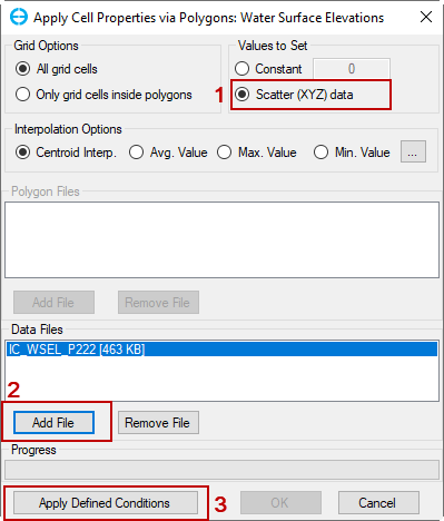
Figure 17.  Assign water surface elevations.

After assigning model water surface elevation, a pop-up will appear to indicate the number of assigned cells and the assigning time.  Click OK in this and all forms to close forms and go back to the Model Control form.

3.4 Assign Boundary Condition Time Series Data

3.4.1 Import flow data series

In this step, we will import inflow data to the EFDC model and then later assign it to the upstream cells. 

1. Expand the External Forcing Data tab on the left side of the Model Control form
2. RMC on Flow
3. Select Add New Data Series from the menu that pops up, as shown in Figure 18

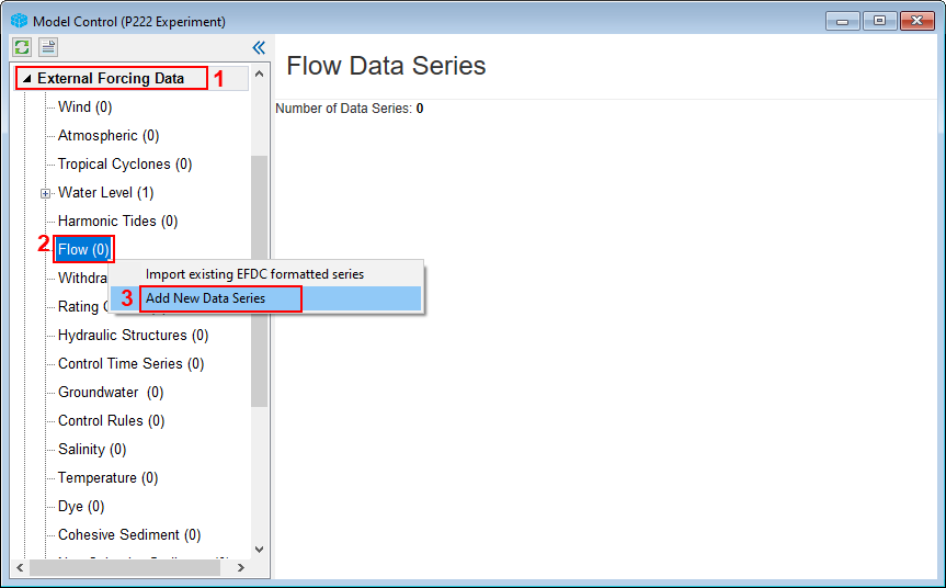
Figure 18.  Assign inflow boundary time series.

The Boundary Data Series form will appear, as shown in Figure 19.  From this form, the user can create new flow boundary time series.

Click on the Add New button to add a new data series, selecting the series named "Inflow”; then add the data shown in Figure 19, below.

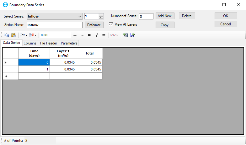
Figure 19. Inflow boundary data series.

After adding the inflow data time series, add a second time series named “Outflow”, as shown in Figure 20.

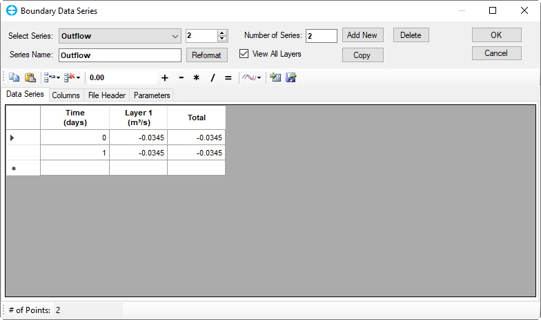
Figure 20. Outflow boundary data series.

3.4.2 Assign Boundary Condition Locations

To assign the boundary condition locations, proceed to the 2DH View form (by clicking on the 2DH View button in the Model Control Form) and under the Layer Control form on the left side of the 2DH View form, do the following:

1. Turn on the editing button of the boundaries layer by clicking on the Boundaries pen icon in the Layer Control frame ( as shown in Figure 21)
2. Select Line Crossing and draw a line through the cells, in this case, along the left side of the grid.

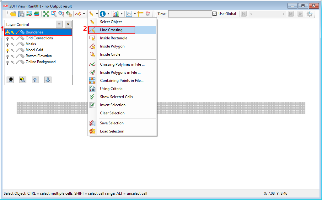
Figure 21.  Edit the boundary layer.

3.RMC on a cell on the left-most cells in the cell map to create the inflow boundary location by then clicking on Add New Boundary Group, as shown in Figure 22. 

4. In the Add BC Group form that appears, type in the Boundary Group Name as “Inflow” and selects the Boundary Group Type as Flow Boundary.

5. Click OK to create the inflow boundary. 

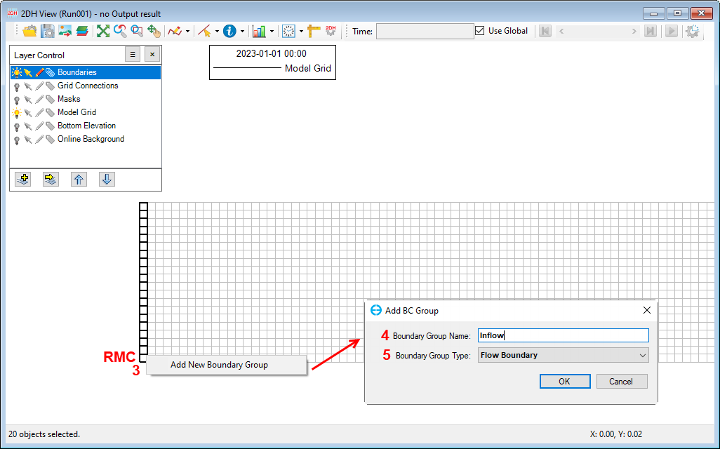
Figure 22.  Assign a boundary location in 2DH View.

The Flow Boundary Conditions form will now be displayed to link the flow table to the BC as shown in Figure 23.

To link the flow series to the BC group, click on the Flow Table drop-down menu in the Forcing Assignment frame and select the Inflow series; then click OK to finish linking the flow series to the BC group and close the form to move forward to the next steps.

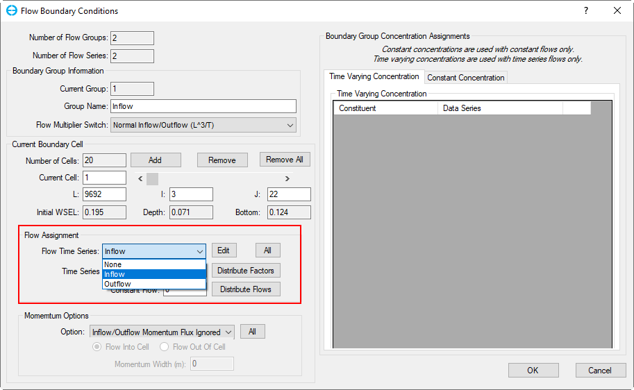
Figure 23.  Link data series to boundary conditions group.

Return to the 2DH View and check to ensure that the assigned boundary locations are correct, as shown in Figure 24.

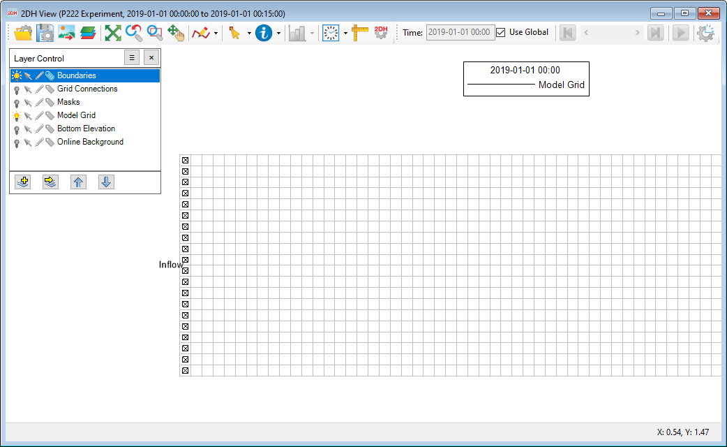
Figure 24.  Inflow boundary locations in 2DH View.

Repeat the same steps for the outflow BC group to assign outflow to the BC group location (refer to Figure 21 and Figure 22) and link the data series to the group (refer to Figure 23 and Figure 24).

1. Select the location to add the outflow boundary, in this case, along the right side of the grid.  RMC on a cell on the rightmost cells in the cell map to create the outflow boundary location by then clicking on Add New Boundary Group (refer to Figure 25). In the Add BC Group form that appears, type in the Boundary Group Name as “Outflow” and select the Boundary Group Type as Flow Boundary. Click OK to create the outflow boundary. 

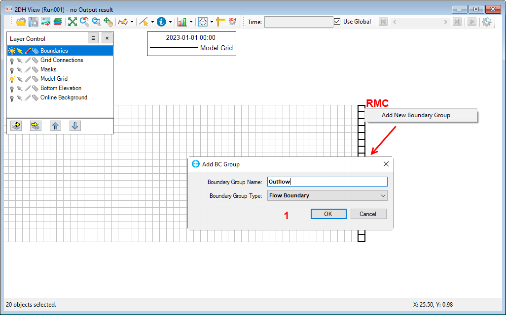
Figure 25.  Outflow boundary locations in 2DH View.

To link the flow series to the BC group, click on the Flow Table drop-down menu in the Forcing Assignment frame, and select Inflow series, as shown in Figure 26; then click OK to finish linking the flow series to the BC group and close the form. Also, link Outflow series as the above steps.

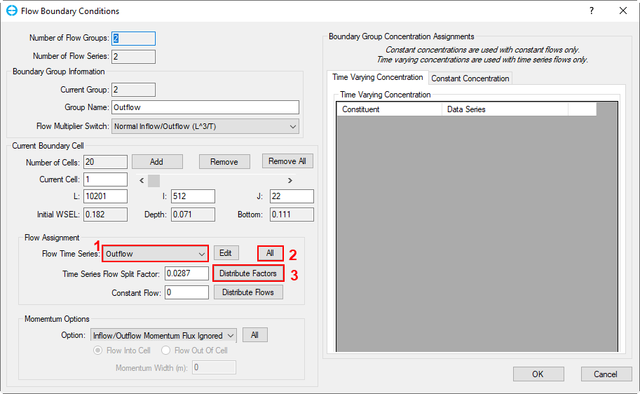
Figure 26.  Link data series to the boundary conditions group.

After that, return to 2DH View and check to ensure that the assigned boundary locations are correct.

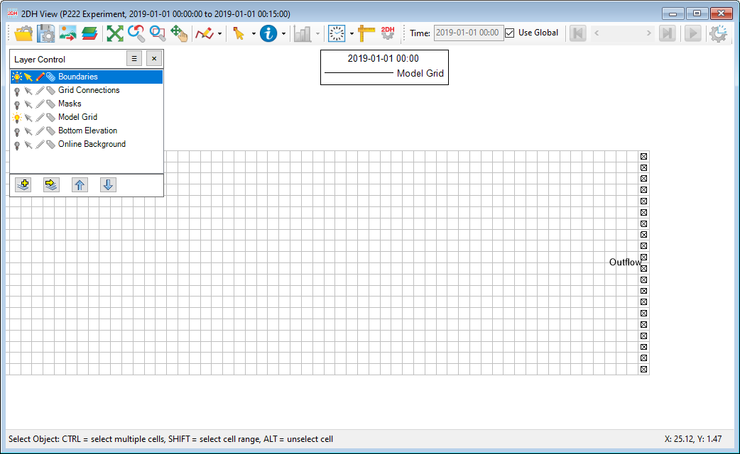
Figure 27. Assigned boundary locations displayed in 2DH View.

3.5  Hydrodynamic Settings

To optimize simulation time and model stabilization, hydrodynamic settings are set as below. 

From the Model Control form,

1. Go to the Modules tab
2. Expand the Hydrodynamics sub-tab
3. RMC on Turbulence to open the Turbulence Options form 
4. From this form, set the Turbulence Diffusion parameters as shown in Figure 28 below.

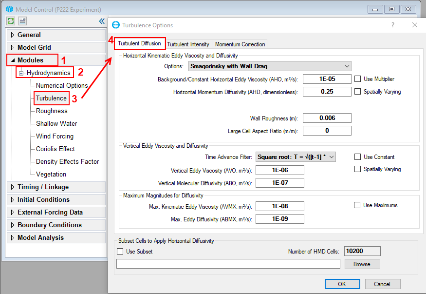
Figure 28.  Hydrodynamics - Turbulence Diffusion settings.

From the Turbulence Diffusion form, go to the Turbulence Intensity tab and then set parameters as shown in Figure 29.  After selecting these settings, click OK to close the form and save the settings.

Note: the settings are retained in the form and in system memory, but you need to save the model for the changes to be written to the EFDC+ input files.

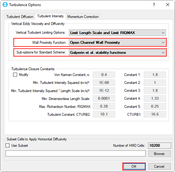
Figure 29.  Hydrodynamics - Turbulence Intensity settings

Next, the user should back to the Model Control form and edit the bed roughness coefficient, as shown in Figure 30.

1. Go to the Modules
2. Expand the Hydrodynamics sub-tab and RMC on Roughness; the Bottom Roughness form will appear.
3. Assign bottom roughness (Z0) as shown in Figure 30. In this test, the average bottom roughness of the model is assigned as 0.0003.
4. Choose EFDC+ 10 and Greater.

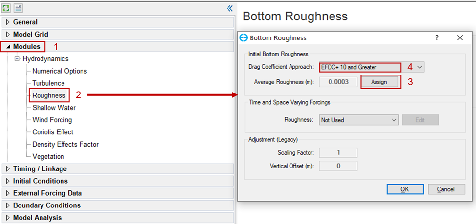
Figure 30.  Hydrodynamics – Assign bottom roughness

Next, to specify shallow water options, from the Model Control form:

1. Go to the Modules
2. Expand the Hydrodynamics sub-tab and RMC on Shallow Water.
3. In the Shallow Water Options, enter the Wet Depth.
4. Enter the Dry Depth and the Dry Step.
5. Choose Use wetting/drying with non-linear iterations and face masking

This feature is required for areas with fluctuating water levels that will leave some of the domain dry.  For an area with tidal flats, users should probably enable the wet and dry option.  Although it incurs a certain computational overhead, this is necessary to obtain accurate results, since it sets the minimum water depth allowed at a point before it is taken out of calculation (Dry Depth), and also the water depth at which the point will be reentered into the calculation (Wet Depth).  In this exercise, shallow water parameters are set as shown in Figure 31.

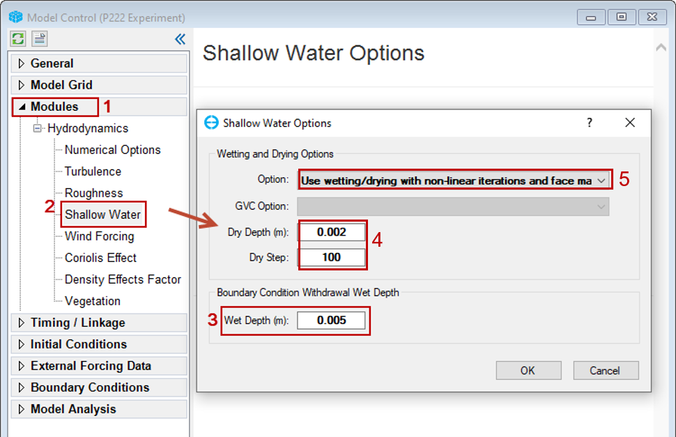
Figure 31.  Hydrodynamics – Shallow Water setting.

Note: The Wet Depth should always be greater than the Dry Depth. 

To include vegetation in the model, the user should go back to the Model Control form and add vegetation, as follows.

1. Go to the Modules tab
2. Expand the Hydrodynamics sub-tab and RMC on Vegetation to open the Vegetation form.
3. The vegetation class settings are available, the user should select the option of Use vegetation with implicit momentum adjustment
4. The vegetation class settings are available via the Modify button option, which provides the Vegetation Class Options form, a user interface to the data needed for the VEGE.INP file.
5. In this example, the user can set up the model with 1 vegetation class by entering the number into the box. The parameters of the vegetation class can be defined as the Figure 32 and then click OK.

The grid will be expanded to accommodate the desired number of classes. All of the inputs required by EFDC+ are shown. The ID and Description are only used by EE. The ID field is used to match vegetation classes to polygon IDs (see the following description of Apply Overlays) to automatically set the vegetation map needed for input via the dxdy.inp file. The Description field is only used for labeling.

Figure 32.  Vegetation model settings.

1. Select the Apply Overlays button uses the vegetation class ID field and matches it to input polygon ID's.
2. Figure 33 shows the form for applying a vegetation map to the model cells. The user should select Only grid cells inside polygons in the grid options.
3. Click Add File to browse the floodplain_Plg.p2d which defines the vegetation location.
4. After that, click Apply Defined Conditions.

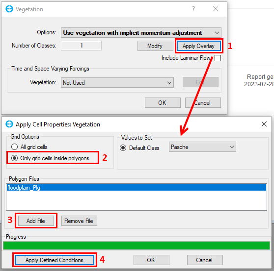
Figure 33.  Apply cell properties via polygon: vegetation.

For more information about Vegetation, please refer to the EFDC+ Explorer Knowledge Base: Vegetation.

3.6 Set Model Timing

After completing the previous sections, the user has almost completed the hydrodynamic model. This section will guide the user on how to set up the model simulation time and model time steps.

1. Select Timing/ Linkage tab and RMC on Timing button (Figure 5‑1)
2. Enter the duration of start/ end of the simulation. Note that the boundaries time series should always cover this simulation duration period, otherwise the model will not run.
3. Enter the Time of Start, Number of Reference Periods, Duration of Reference Periods and Time Step as Figure 34. These values are explained detail in Simulation Timing Options

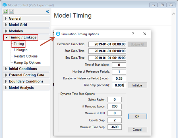
Figure 34.  Simulation Timing settings.

4. Returning to the Model Control form, expand Timing/Linkage on the left and RMC on Linkages (Figure 3‑34) to set the output frequency. In the EFDC Model Linkages form that pops up, select Link EFDC Results to EFDC+ Explorer in the EFDC+ Explorer Linkage tab and frame, and set the Linkage Output Frequency.  In this exercise, set Linkage Output Frequency to 0.25 minutes.  This means EFDC will record the output every 0.25 minutes for displaying. 

Note: The smaller the output frequency, the larger the output file size.

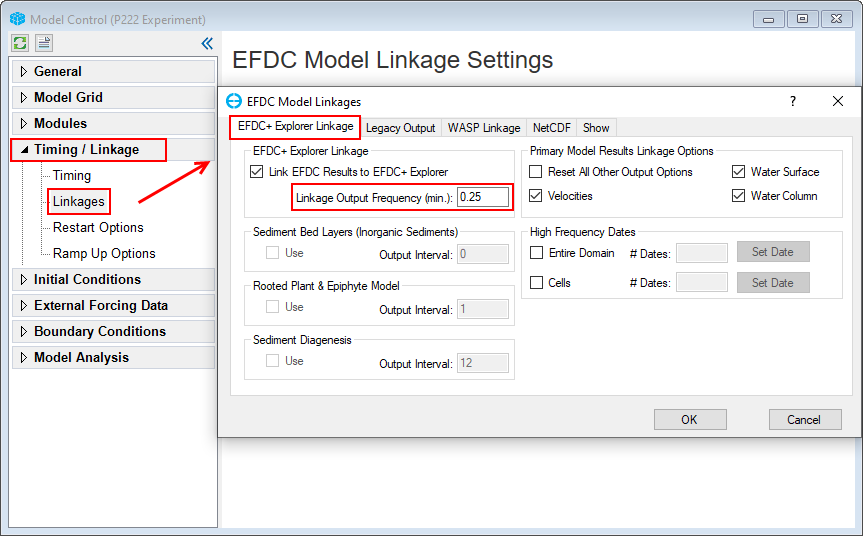
Figure 35.  EFDC Explorer Model Linkage Setting form.

5.Click on the OK button to save the model.

3.7 Model Runs

Back to the main form, click this button to run the model. The EFDC+ Run Options form will appear; Figure 36. in this form, under the General tab, set the OMP per Domain to use for the EFDC+ run.   Note that #OMP Cores Used for EFDC+ run must be smaller than the Available CPU Cores.

Browse to the EFDC+ executable file and select the updated executable file.

Note: If the model has existing results, please check on the Overwrite check box to run and save new results. 

Click on the Run EFDC+ button to start running the model.

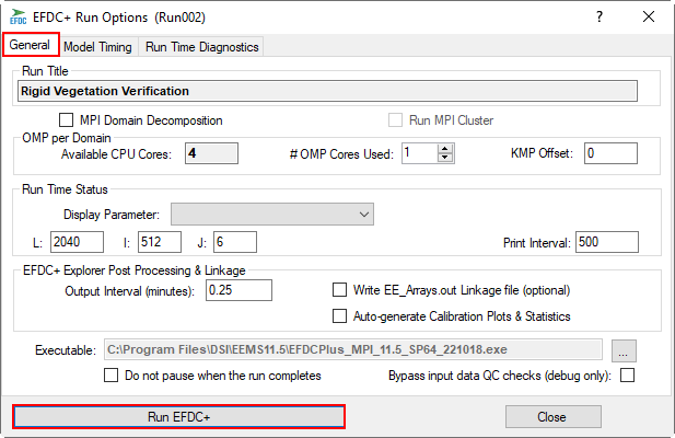
Figure 36. EFDC+ Run Options form.

A run window such as that pictured in Figure 37 will appear.

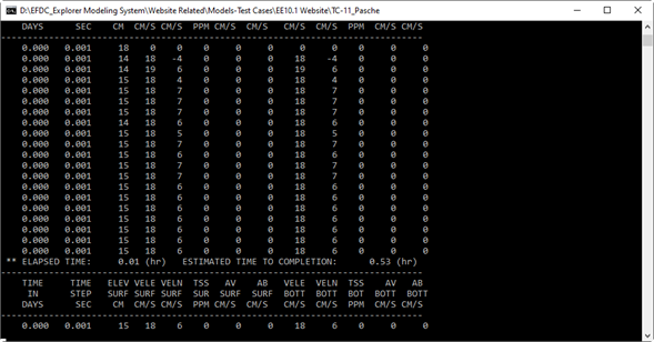
Figure 37.  EFDC+ run window.

4. Step-by-Step Guide for Model Output Visualization

4.1 Model Output Visualization

After each simulation run finishes click on the Refresh Output button in the toolbar to refresh the model output ( as shown in Figure 38).

Figure 38.  Refresh Button in the Model Interface

Take the following steps to visualize the model output:

1. Click the 2DH button to bring up the 2DH View window.
2. In the Layer Control frame, click on the Add New Model Layer button to open the 2DH View Option form, which is used to select a layer to add to 2DH View. 
3. Select the desired parameter to add to the 2DH View in the Primary Groups and Parameters drop-down menus; in this case, the selected parameter is Vegetation Density. 
4. Click on the Add button to add the layer to the 2DH View (Figure 39). 

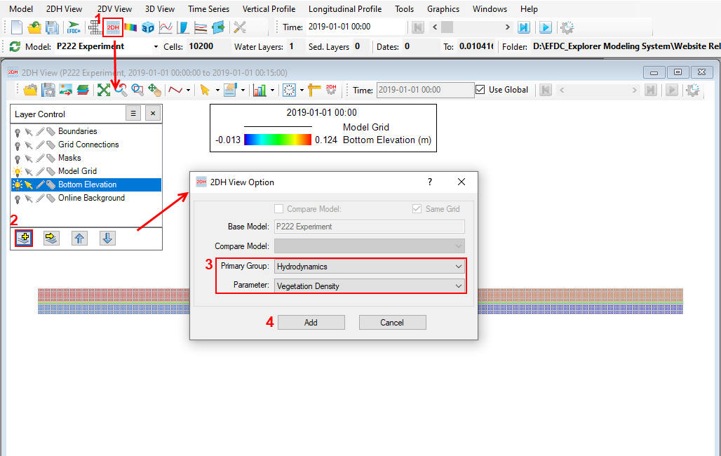
Figure 39.  Visualize model output in 2DH View. 

5. To modify the settings of layer properties displayed on the legend, RMC the layer (in this case, Vegetation Density).  The pop-up that appears will offer various options to edit, as shown in Figure 40.

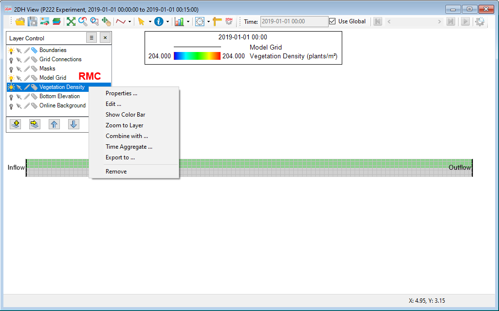
Figure 40.  Edit layers in 2DH.

For more information about Layer Properties Settings in 2DH View, please refer to the EFDC+ Explorer Knowledge Base: Layer Properties Settings

4.2 Model Verification

To verify the model, the user can extract simulated profile velocities from a cross-section at 20 m (col: I=403) and compare them with measured data points.

1. In the main toolbar, click on Longitudinal Profile in the main toolbar and the select New Longitudinal Profile.  The Data Extraction for Longitudinal Profile form will appear, as shown in Figure 41.
2. In the Profile Definition frame, select Use I and then Specify I as a cross-section of 403.
3. In the Define Parameter to Plot frame, select Velocity Magnitude, then click Update The velocity magnitude of the selected cell will be extracted.

Figure 41.  Data extraction for a longitudinal profile.

4. To compare the measured and simulated velocity, select the Import Data button from the main toolbar and select the “Measured data_Pasche P222.dat” file to load into the “Data” folder, as shown in Figure 42.

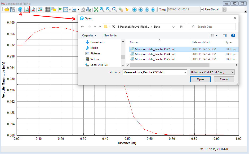
Figure 42.  Add measured velocity to compare.

When the measured data is added, edit the plot. RMC on the legend to change the display of measured velocity to a symbol by checking the Show Symbols box in the Data Series frame that appears ( as shown in Figure 43). Finally, compare the simulated velocity and measured velocity at a certain time; a close correlation between the simulated and measured velocities verifies the model with respect to this parameter.

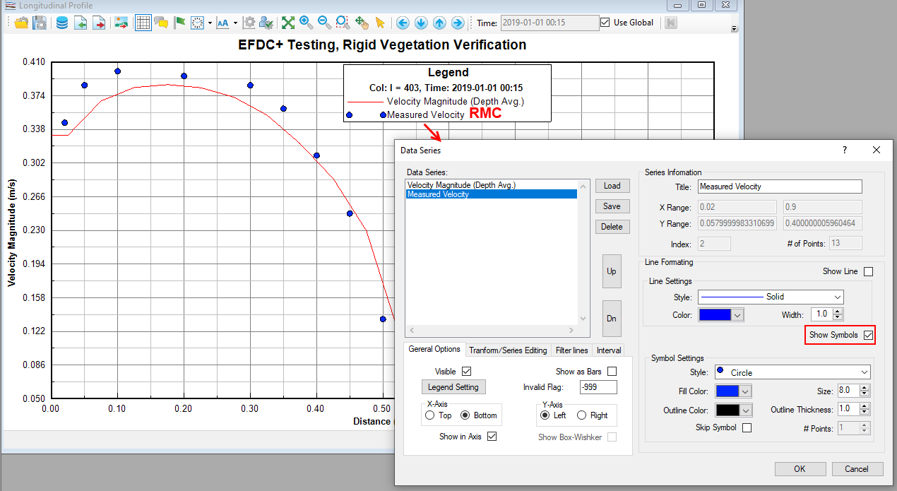
Figure 43.  Edit the data plot.

5. Scenario Modeling

5.1 Changing Vegetation Density

Return to the Model Control form and adjust the vegetation as follows:

1. Go to the Modules tab
2. Expand the Hydrodynamics sub-tab and RMC on Vegetation to open the Vegetation form. 
3. The vegetation class settings are available via the Modify button option, which provides the Vegetation Class Options form, a user interface to the data needed for the VEGE.INP file.
4. Adjusts the plant density as shown Figure 44.

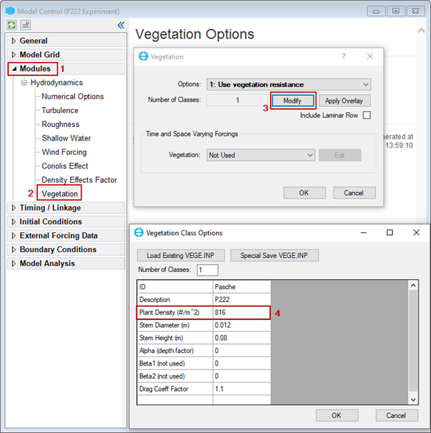
Figure 44.  Increase plant density.

Click on the OK button to save the model.

To run the model, follow the steps shown earlier in Figure 36.

After each simulation run finishes click on the Refresh Output button in the toolbar (as shown in Figure 38) refresh the model output.

In order to analyze the impact of changing vegetation density, take the following steps to visualize the model output:

1. Click the 2DH button to bring up the 2DH View window.
2. In the Layer Control frame, click on the Add New Model Layer button to open the 2DH View Option form, which is used to select a layer to add to 2DH View. 
3. Select the desired parameter to add to the 2DH View in the Primary Groups and Parameters drop-down menus; in this case, the selected parameter is Vegetation Density. 
4. Click on the Add button to add the layer to the 2DH View (Figure 45). 

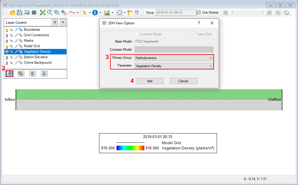
Figure 45.  2DH View form showing vegetation density.

You are now able to see that the vegetation density currently is 816 plant/m².

To verify the model, extract the time series of the simulated total bed shear from a cross-section (L=8284, I= 125, J=19) and compare them with the original model.

1. In the main toolbar, click on Time Series Plot.  The Extract Time Series Data form will appear, as shown in Figure 46.
2. In the Selected Cells frame, select cell L=8284.
3. In the Define Parameter to Plot frame, select Total Bed Shear, then click Update The total bed shear of the selected cell will be extracted.

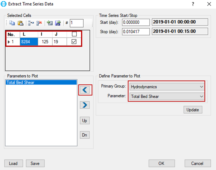
Figure 46.  Extract total bed shear.

The time series plot of total bed shear is shown in the Figure 47 below.

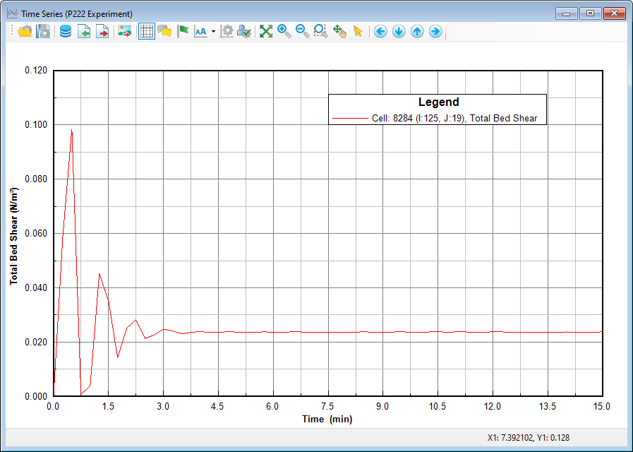
Figure 47.  Time series of total bed shear of the high-density model.

To extract data to compare with the total bed shear of the original model:

1. Click Export Data Series as shown in Figure 48
2. Browse to the file location and save the file.

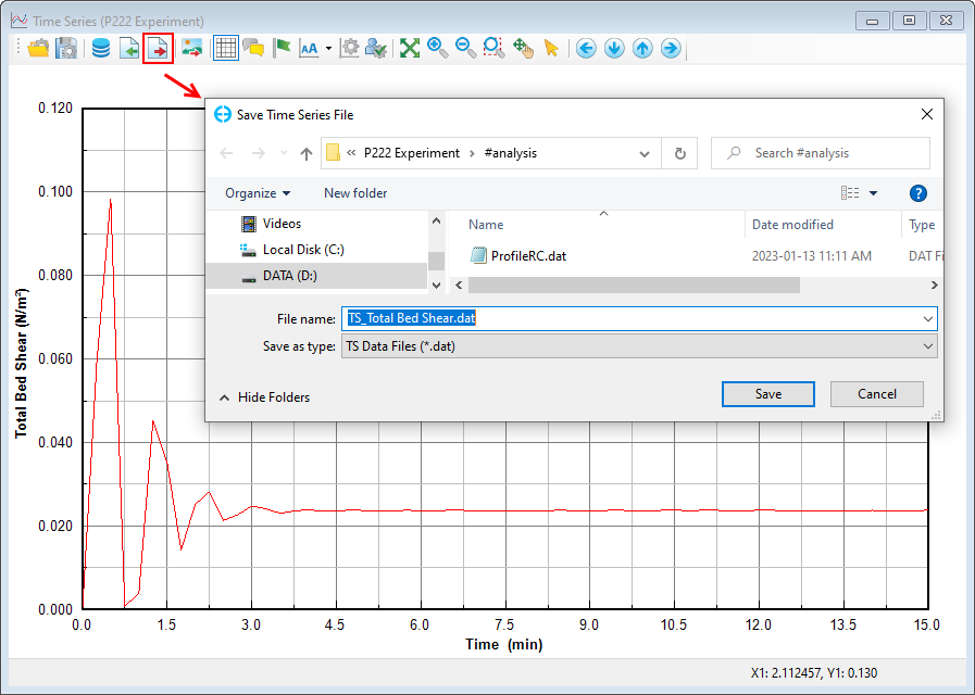
Figure 48.  Export time series data.

Carry out similar steps to decrease the parameter of vegetation density as shown in Figure 49.

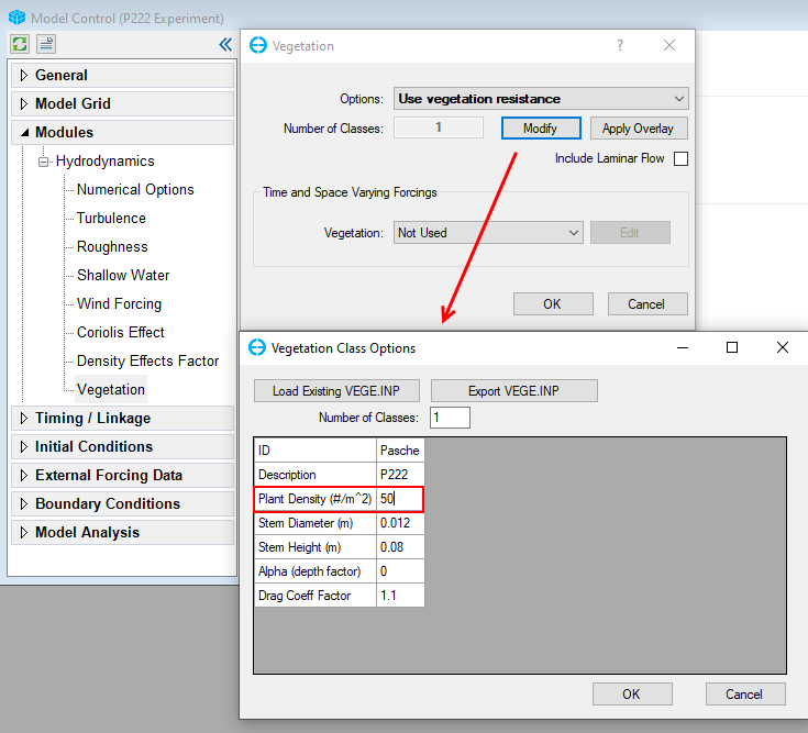
Figure 49.  Decrease plant density.

And then save and run the model again. Carry out similar steps again as shown in Figure 48 to extract the total bed shear for the same cell (L=8284, I= 125, J=19).

In the main toolbar, click Import Data Series and browse to the total bed shear of the original model.

You are now able to compare the difference in the total bed shear of the original model with the high plant density and low plant density as shown in Figure 50.

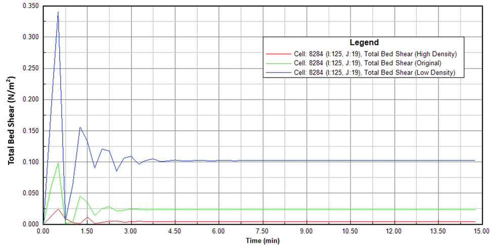
Figure 50.  Total bed shear comparison of changing density model.

To further verify the model, extract the longitudinal profile of the velocity magnitude from a cross-section at 20 m (col: I=403) and compare them with the original model.

In the main toolbar, click on Longitudinal Profile as shown in Figure 51.

Figure 51.  Longitudinal profile.

1. In Profile Definition, check Use I and specify I=403 ( as shown in Figure 52)
2. In the Define Parameter to Plot frame, select Velocity Magnitude, then click Update The velocity magnitude (depth average) of the selected cell will be extracted.

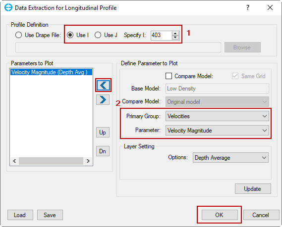
Figure 52.  Data extraction for a longitudinal profile.

Carry out similar steps to extract the longitudinal profile of velocity magnitude at the same cross-section (col: I=403) of the low-density and high-density model to compare with the original model.

Figure 53 illustrates the velocity magnitude of the original model and low- and high-density models at the cross-section I=403.

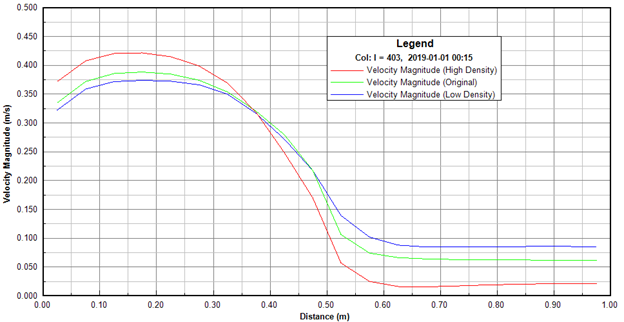
Figure 53.  Velocity magnitude comparison of changing density model.

It can be observed in Figure 53, when the plant density increases the velocity magnitude in the main channel climbs while the floodplain area shows a decline in the velocity magnitude. 

5.2 Decrease Vegetation Height

Return to the Model Control form and adjust vegetation, as follows.

1. Go to the Modules tab
2. Expand the Hydrodynamics sub-tab and RMC on Vegetation to open the Vegetation form. 
3. The vegetation class settings are available via the Modify button option, which provides the Vegetation Class Options form, a user interface to the data needed for the VEGE.INP file.
4. Adjust the stem height as Figure 54.

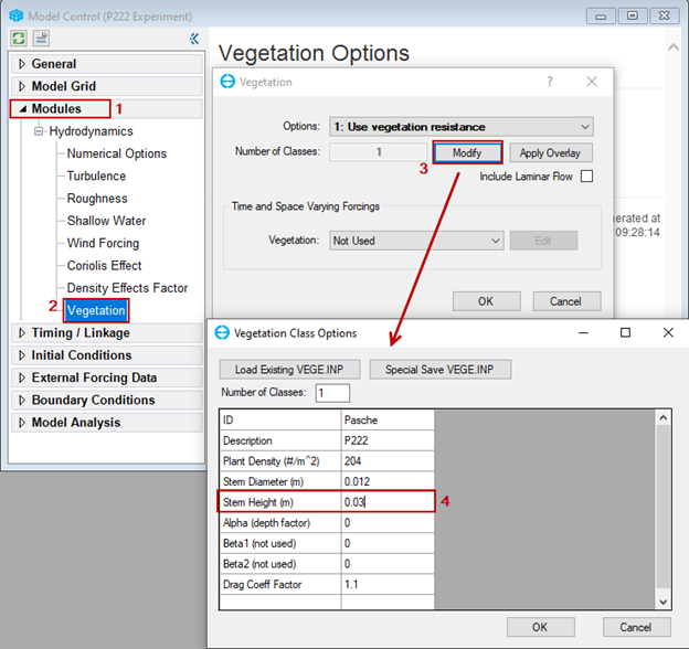
Figure 54.  Decrease stem height.

Click on the OK button to save the model.

To run the model, follow the steps above, as shown in Figure 37.

After each simulation run finishes click on the Refresh Output button in the toolbar to as shown in Figure 38 refresh the model output.

In order to observe the impact of changing vegetation height, take the following steps to visualize the model output:

1. Click the 2DH button to bring up the 2DH View window.
2. In the Layer Control frame, click on the Add New Model Layer button to open the 2DH View Option form, which is used to select a layer to add to 2DH View. 
3. Select the desired parameter to add to the 2DH View in the Primary Groups and Parameters drop-down menus; in this case, the selected parameter is Vegetation Height. 
4. Click on the Add button to add the layer to the 2DH View (Figure 55). 

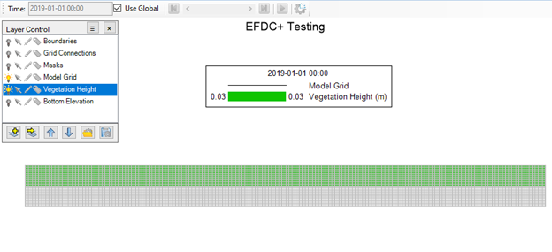
Figure 55.  2DH View form showing vegetation height.

You can now see that the modified vegetation height is 3cm.

Carry out similar steps to extract the data of total bed shear to compare with the original model at the same cell (L=8284, I= 125, J=19).

Figure 56 shows the total bed shear of the original model with decreased stem height model.

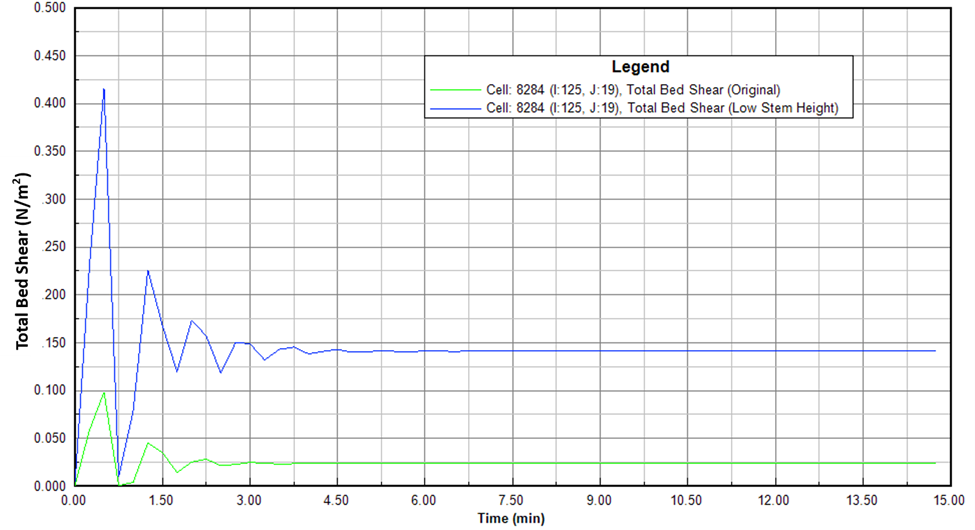
Figure 56.  Total bed shear comparison of decrease vegetation height.

Carry out similar steps to extract the longitudinal profile of velocity magnitude at the same cross-section (col: I=403) of the decreased stem height model to compare with the original model.

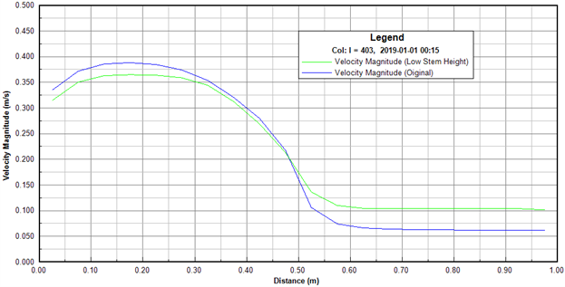
Figure 57.  Velocity magnitude comparison of decrease stem height model.

From Figure 57,  it can be seen that when the height of the plant reduces the flow in the floodplain also decreases. Meanwhile, the flow in the main channel goes up.