Build a 3D Lake Model with Sigma Zed (Level 2 Step-by-Step Guidance)
Introduction
Lake Washington is a large freshwater lake adjacent to the city of Seattle and the largest in King County. It is a ribbon lake, 35 km long and surface area of approximately 88 km2. Mercer Island lies at the southern end of the lake. The main inflows are from the Sammamish River in the north and Cedar River in the south. The outflow is to via a ship canal at Puget Sound in the west with the discharge of approximately 7 m3/s.The bathymetry of Lake Washington shows that it is a deep, narrow, glacial trough with steeply sloping sides and approximately 65 m deep at its deepest point. These morphologic features are highly suitable for the application of the SGZ model.
This tutorial document will guide you on how to set up a Sigma Zed model by using the EFDC+ Explorer (EE). It will cover the preparation of the necessary input files for the EFDC model and visualization of the output by using the EFDC+ Explorer (EE) Software.
The data used for this tutorial are from Lake Washington. All files for this tutorial are found in Lake Washington model downloadable from the EE website.
Before going to each session, let’s first introduce the main form of EE User Interface in order to better understand our explanation hereafter. Figure 1 is the main form of EFDC+ Exploreror EE User Interface. Functioning for individual icons are described as following;
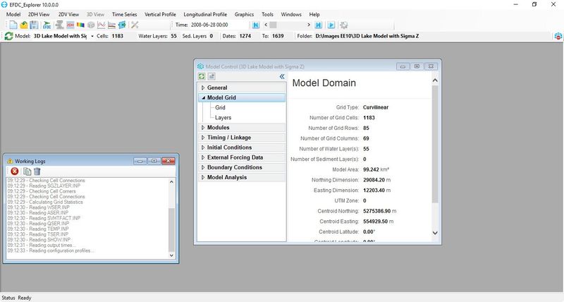
Figure 1. EFDC+ Explorer Main Form.
2 Import Grid
This session will guide you to import the grid into EFDC+ Explorer. With a complicated grid such as this, the grid generation software CVLGrid is required to been used. Lake Washington in Washington state, the USA has been chosen as an example of building a 3D Lake Model with Sigma Zed in EE.
The grid generation process includes the following steps:
- Open EE
- Click New Model icon as
 on the main menu of the EE interface. Then Grid Tool frame appears shown in Figure 2.
 - Select Import Grid from Files option then click Import Grids button. The Import Grid form appears, the select CVLGrid in Grid type, then click Browse button to select grid file name as "LW Grid.cvl" as shown in Figure 2 then click OK button. Note that EE also supports importing a variety of grid formats with the option Import Grid shown in Figure 3.
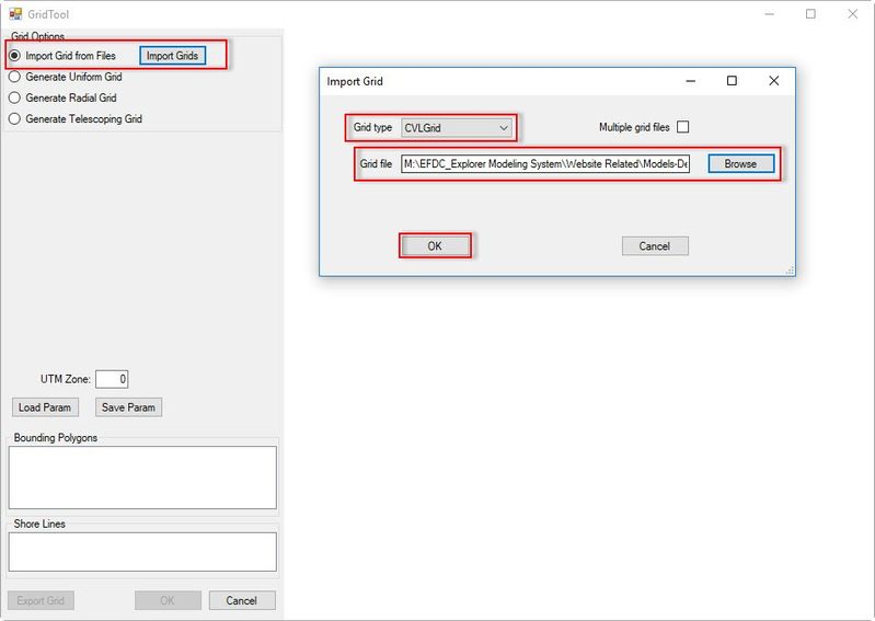
Figure 2. Generate EFDC Model form.
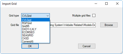
Figure 3. Import grid options.
4. Click OK button, the imported grid is shown (Figure 4).
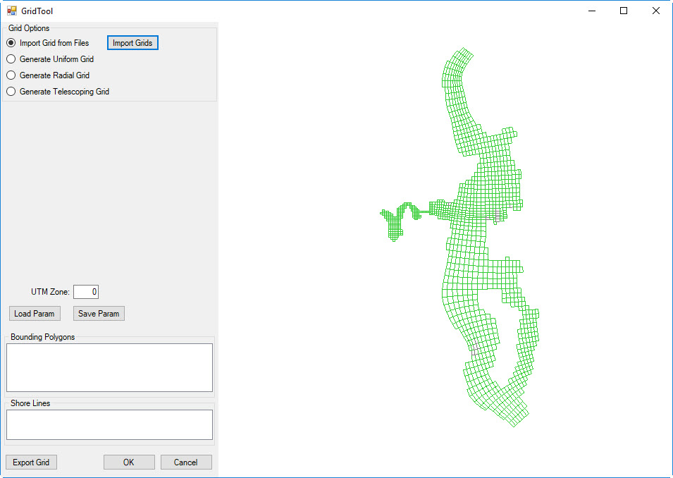
Figure 4. Newly imported grid.
5. Save the model by selecting this button  and create a new directory as shown in Figure 5.
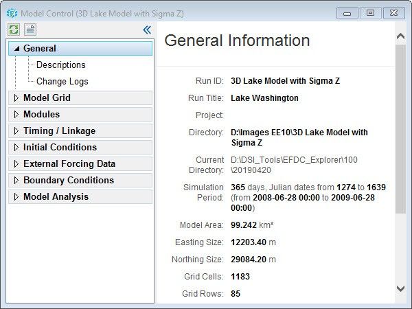
Figure 5. New model saved.
3 Assigning the Initial Conditions
This section will guide you on how to assign the initial conditions such as the bathymetry, water level, and bottom roughness.
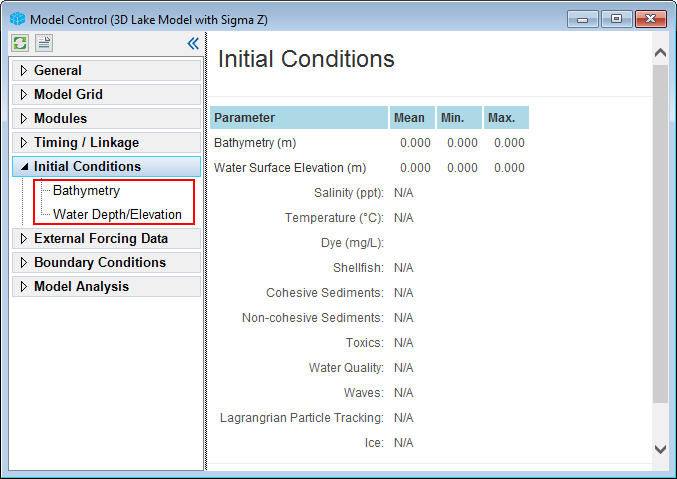
Figure 6. Assigning the Initial Conditions.
3.1 Assigning the Initial Bottom Conditions
- Select the Initial Conditions section and RMC on the Bathymetry. A form will be displayed as shown in Figure 7.
- In the Bathymetry windows click on Assign button to open Apply Cell Properties via Polygons: Bottom Elevation windows.
- In Grid Option choose All grid cells, in Values to set choose Scatter (XYZ) data. In the below text box of Scatter data file, click on Add file button to browse to the bathymetry file XXXXX. This bathymetry file is simply a general x,y, z format.
- In this case, we choose Interpolate Options is Centroid Interp. and It means that it will take the surrounding data points to interpolate for the cells where the data is not available.
- Note that Poly File is the area to assign the bathymetry data.
- Click the Apply Defined Conditions button to take the effect before hitting the OK button.
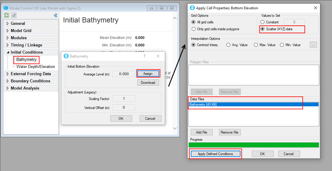
Figure 7. Assigning model bathymetry.
3.2 Assigning the Depth/Water Surface Elevations
The next step is to assign the initial depth or water surface elevations. There are also two options for setting the surface water elevation that is Use Constant and Use Scatter (XYZ) data. In this case, we will use the former option.
- Select the Initial Conditions section and RMC on the Water Depth/Elevation. A form will be displayed as shown in Figure 8.
- In the Water Depth/Surface Elevation windows click on Assign Elevation button to open Apply Cell Properties via Polygons: Water Surface Elevation windows.
- In Grid Option choose All grid cells, in Values to set choose Constant and type the value equal to 6.5 on the beside text box.
- Click the Apply Defined Conditions button to take the effect before hitting the OK button.
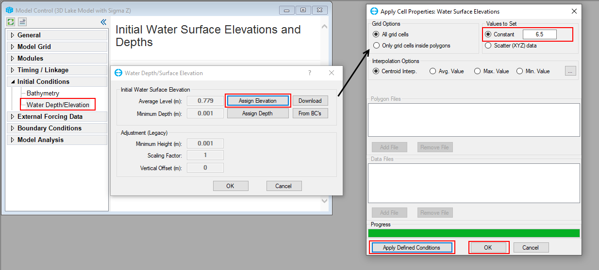
Figure 8. Assigning water surface elevation.
3.3 Assigning the Bottom Roughness (Z0)
- Select the Initial Conditions section and RMC on the Roughness. A form will be displayed as shown in Figure 9.
- In the Bottom Roughness windows click on Assign button to open Apply Cell Properties via Polygons: Bottom Roughness windows.
- In Grid Option choose All grid cells, in Values to set choose Constant and type the value equal to 0.02 on the beside text box.
- Click the Apply Defined Conditions button to take the effect before hitting the OK button.
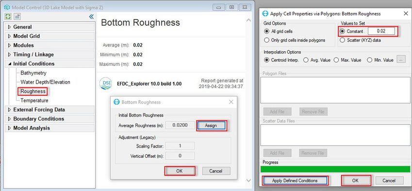
Figure 9. Assigning bottom roughness.
4 Assigning the Boundary Conditions
This next step is to prepare for the boundary conditions and assign these to the model grid. In this model, there are seven flow boundaries, all but one of which are rivers flowing into Lake Washington. The Lock BC is an outflow. Figure 10 shows flow boundaries of the model.
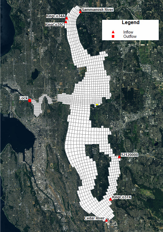
Figure 10. Inflow and outflow of Lake Washington.
4.1 Preparing the Flow Boundary
- Select the External Forcing Data section (Figure 11).
- RMC on Flow and select Add New Data Series to edit the flow boundary (Figure 11).
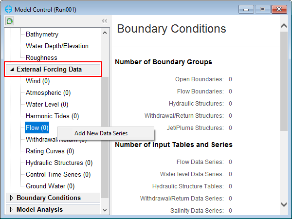
Figure 11. Assigning Flow Boundary Conditions.
3. Enter the Number of Series into the box. There are seven flow boundaries as mentioned so it should be “7”.
4. Give a Series Name for associated time series (remember to press Enter after each input).
5. Select Import Data from File button and then browse to the inflow data file as shown in Figure 12.
6. Click Preview/Graph to view the current time series (Figure 12).
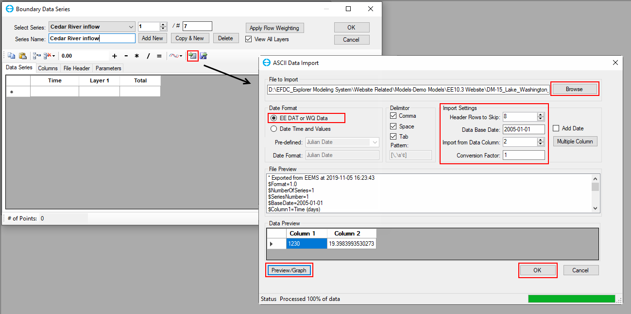
Figure 12. Editing the Boundary Time Series.
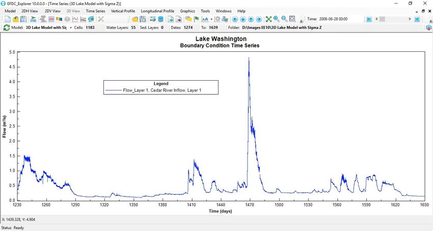
Figure 13. Flow Time Series Plot.
7. Change up/downward this ![]() button to edit other time series.
button to edit other time series.
8. Click OK to finish editing the flow boundary time series.
4.2 Preparing Temperature Boundary
- In Model Control windows, RMC on Modules section to open the EFDC Modules windows.
- Click on the checkbox of Temperature to enable the Temperature module and press OK to finish (Figure 14).
- Select the External Forcing Data section (Figure 11).
- RMC on Temperature and select Add New Data Series to edit the temperature boundary.
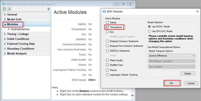
Figure 14. Enable Temperature module.
3. Enter the Number of Series into the box. There are three temperature boundaries as mentioned so it should be “3”.
4. Give a Series Name for associated time series (remember to press Enter after each input).
5. Copy and paste time series data into the workspace corresponding to each series. Figure 12 shows time series of Cedar River temperature.
6. Go to the Time series plot menu and click on View series to view the current time series (Figure 12). For a case where there are multiple layers, please click on View Option at below to choose the way to analyze multiple layers (Sum layer for total flow, Average layer for average flow or Custom for specific layers).
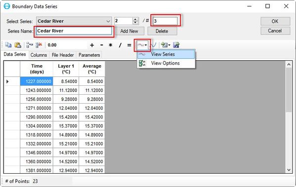
Figure 15. Editing the Boundary Time Series.
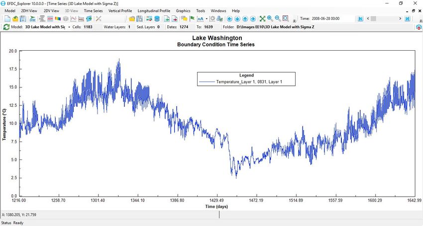
Figure 16. Temperature Time Series plot.
4.2 Preparing Wind Boundary
- Select the External Forcing Data section.
- RMC on Wind and select Add New Data Series to edit the wind boundary. (Figure 17)
- Enter the Number of Series (Type 1) (Figure 18).
- Give a Tittle for associated time series.
- Select Import data from File and browse Wind data time-series (Figure 18).
- The user can edit the parameters of the wind station by clicking on Parameters tab (Figure 19).
- The user can view wind rose by clicking Wind Rose button (Figure 20).
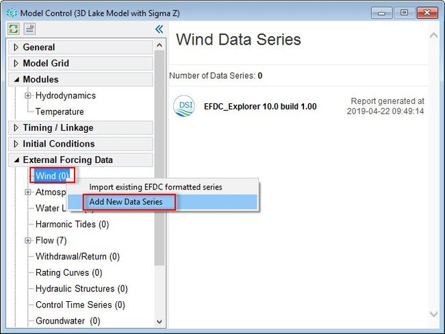
Figure 17. Assigning Winds Boundary Conditions.
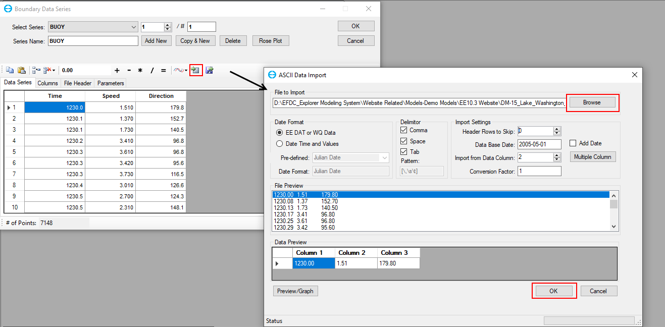
Figure 18. Editing the Boundary Time Series.
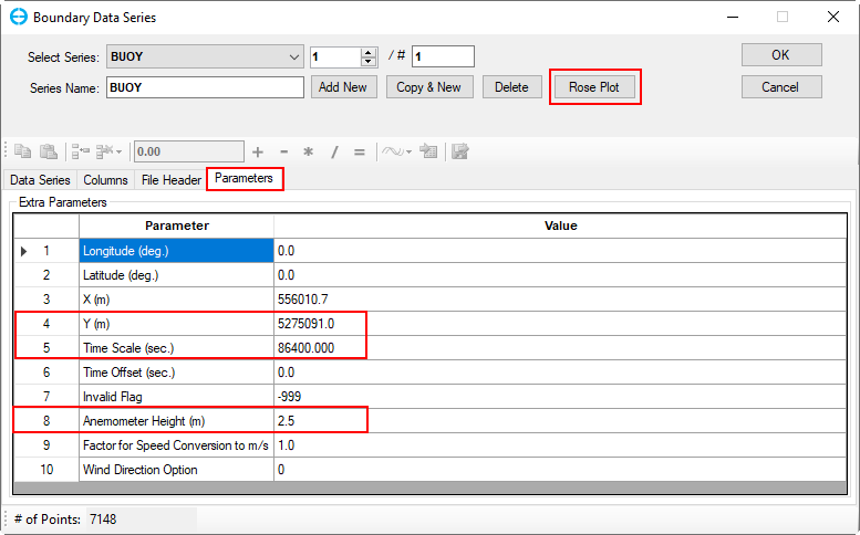
Figure 19. Editing Wind Station Parameters.
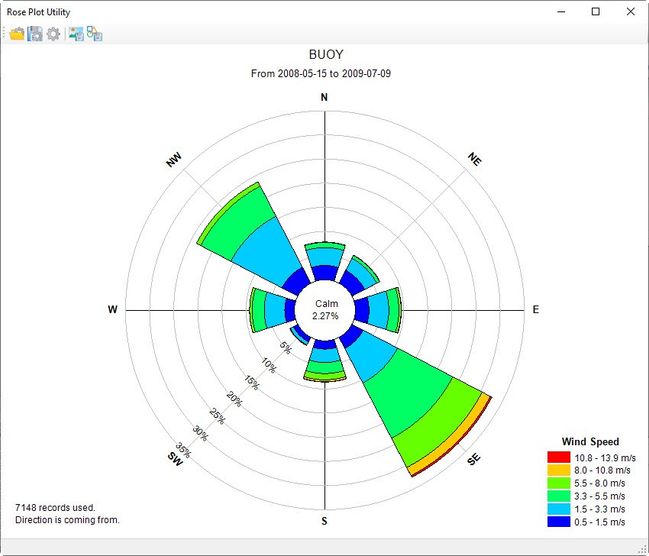
Figure 20. Wind Rose.
4.3 Preparing Atmospheric Boundary
- Select the External Forcing Data section.
- RMC on Atmospheric and select Add New Data Series to edit the wind boundary (Figure 21).
- Enter the Number of Series (Type 1) (Figure 22).
- Give a Tittle for associated time series.
- Select Import data from File and browse to the atmospheric time-series. Please note that the user needs to select import multiple columns and data import settings should be set as Figure 22.
- The user can edit the parameters of the ATM station by clicking on Parameters tab (Figure 23).
- Go to the Time series plot menu and click on View series to view the current time series (Figure 24). User can click on View Option below to choose which parameters can show up.
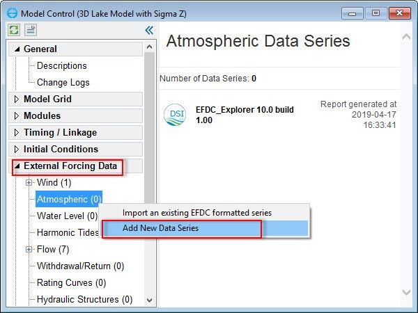
Figure 21. Assigning Atmospheric Boundary.
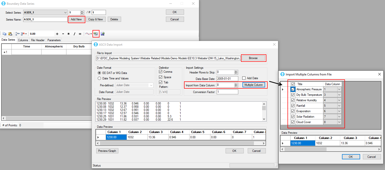
Figure 22. Editing the Boundary Time Series.
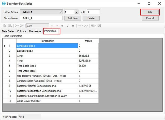
Figure 23. Editing ATM Station Parameters.
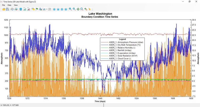
Figure 24. Viewing ATM Data.
4.4 Assigning Time Series to the Boundary Location Cells
When all required boundary time series are prepared the user must assign those boundary time series to the model cells.
In order to assign the flow boundary, the following steps should be taken:
1. Click to the 2DH View menu item or icon 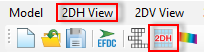 on the main form (Figure 1).
2. Choose Boundaries in the View Layer Control by clicking on the light icon ![]() .
.
3. Enable Edit grid by turning on the icon ![]() (Figure 25).
(Figure 25).
4. In order to know locations of cells assigned flow BC, the user should load the labels file (BC Location.dat). Go to Import an External Overlay Layer button at the bottom Layer Control from then select the label file and remember to choose the type of import file as Label Files (*.lbl, *.dat, *.txt), then load the label file as shown in Figure 26 and Figure 27.
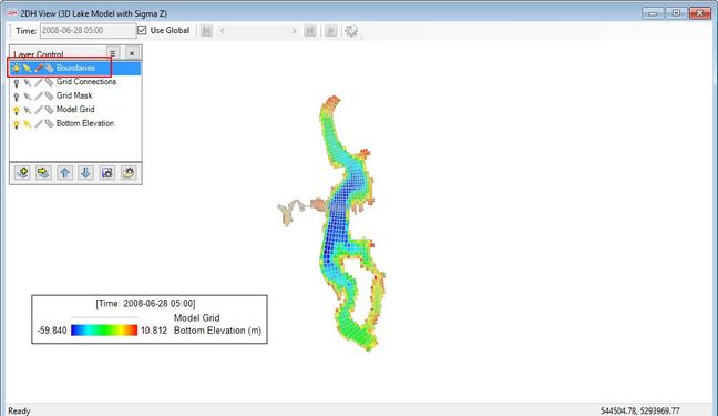
Figure 25. Assigning Boundary Condition Cells.
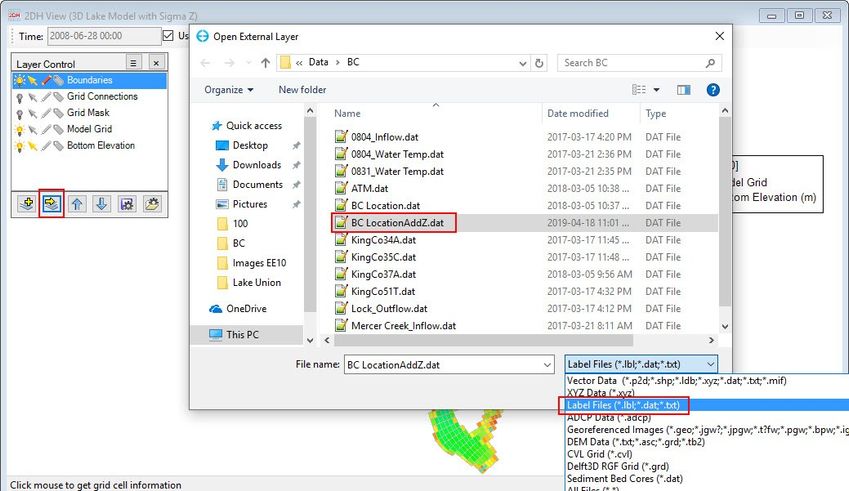
Figure 26. Loading Label File.

Figure 27. Labels Displayed
5. Zoom in to each label location then RMC on the inflow/outflow location cell and click on New (Figure 28).
6. Enter the boundary group ID: Inflow group (Figure 29).
7. Select boundary types. It is dependent on your current boundary condition to choose the suitable boundary type. In this case, we choose Flow Boundary (Figure 29).
8. Select the associated with this inflow boundary time series (Figure 30) then click OK to complete.
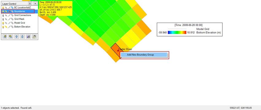
Figure 28. Right-Mouse-Click on the inflow cell.
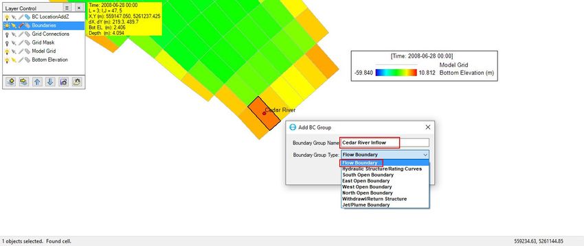
Figure 29. Enter Boundary Group Name and Select the Boundary Types.
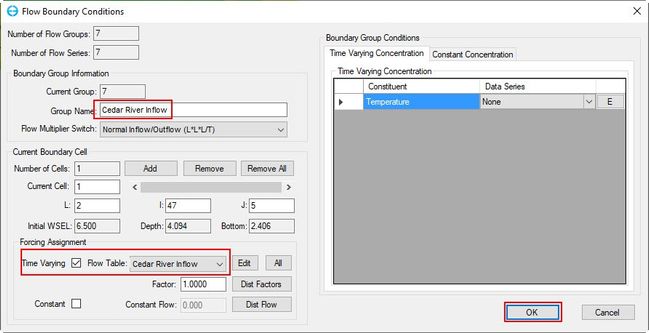
Figure 30. Assign the Corresponding Time Series.
9. The boundary cells often have multiple cells to represent the real river width. In order to assign the next cell as an inflow cell, return to step 5 and RMC that cell and choose Add Cell to Adjacent Boundary Group. The inflow is now divided across the number of assigned cells (Figure 31).
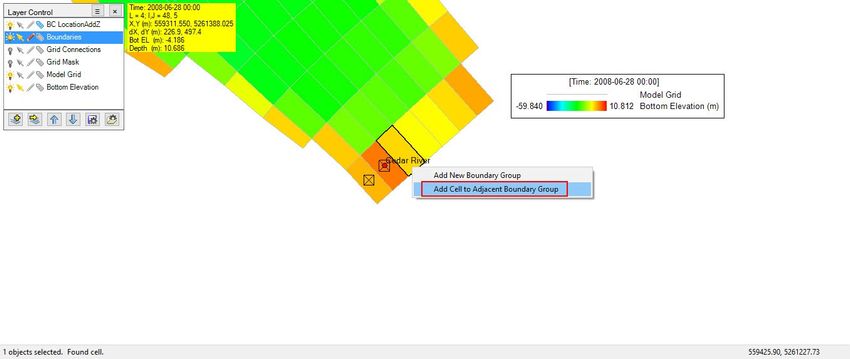
Figure 31. Assign more boundary cells.
10. Select all boundary cells by pressing the Shift key and clicking on all boundary cells (3 cells in this case), then RMC on one of them, and select Edit Boundary Cells (Figure 32).
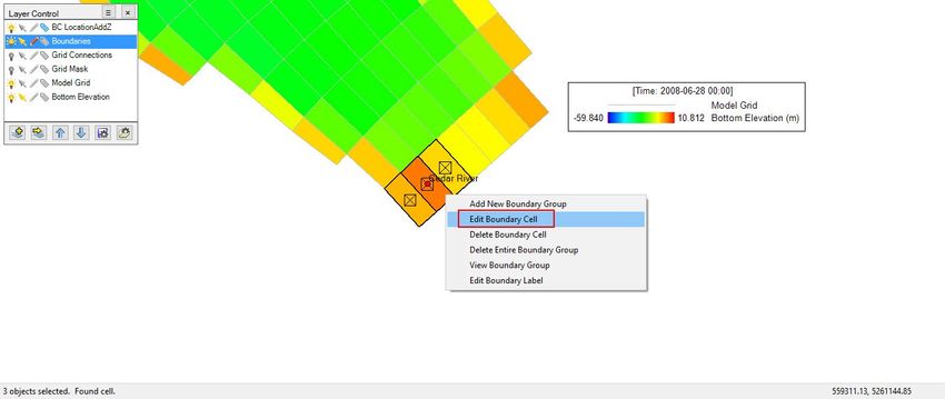
Figure 32. Right-Mouse-Click on the inflow boundary cells.
11. Click on Dist Factors to divide the flow across the 3 cells (See Figure 33) and press OK to finish.
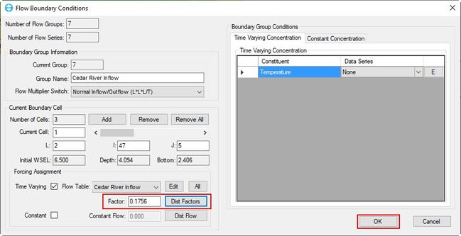
Figure 33. Distribute all inflow boundary cells of the Cedar River group.
12. Carry these same steps above for the remaining flow boundaries.
The temperature boundary is associated with the flow boundary, in this case there two temperature boundaries, one is associated with Cedar River inflow and the other is related to Sammamish River inflow. The following steps should be taken:
- Reopen Flow Boundary Conditions that introduced in the above steps (Figure 33).
- In the Boundary Group Conditions section on the right, the user can choose the Data series corresponding to the Flow group, for example, temperature table 0831 belongs to Cedar River Inflow and 0804 belongs to Sammamish River (See Figure 34).
- Click OK button to finish.
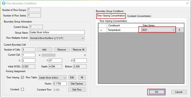
Figure 34. Assign temperature boundary.
5 Setup Grid Layers (Sigma Zed)
- In the Model Control window, click to Model Grid section then RMC on Grid or Layers to open the Model Grid form (Figure 35 and Figure 36).
- Choose SGZ: Specified Bot Layer in the Water layers section on the right.
- Enter the number of water layers. In this case, this is 55 then press Enter (Figure 36).
- Click Set SGZ Layering, and the form will appear as shown in Figure 36.
- Put KMin = 2 for the minimum number of layers, then click OK button.
- Cell information will be updated as shown in Figure 37.
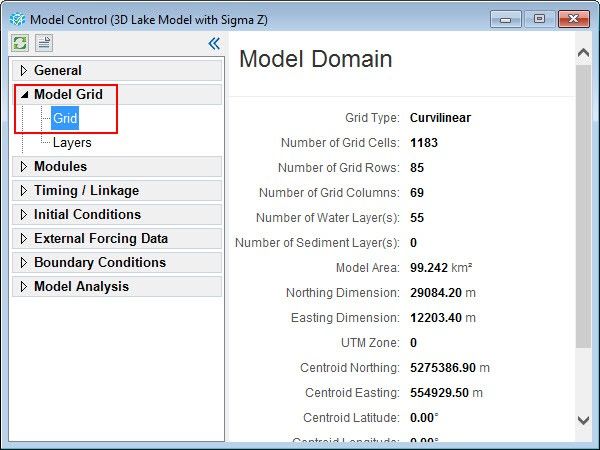
Figure 35. Open Model grid windows.
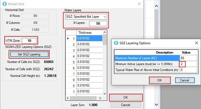
Figure 36. SGZ Layering Options Form.
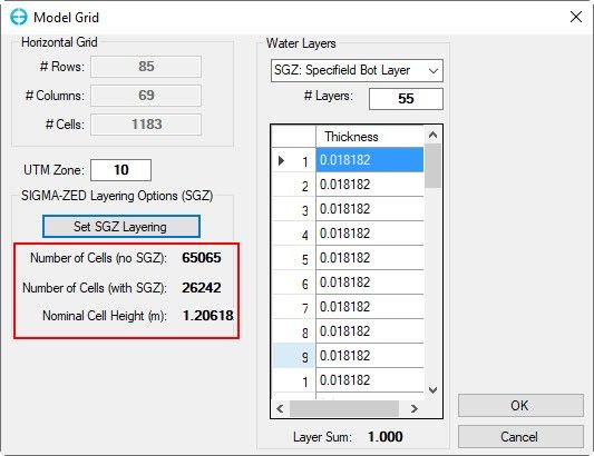
Figure 37. SGZ Layering Options Information.
6 Initial Conditions and Options for Water temperature module
RMC on Temperature menu item in the Modules section and click on Settings, to open the Temperature Parameters form as shown in Figure 39. Set the initial conditions for each tab as shown in the following figures:
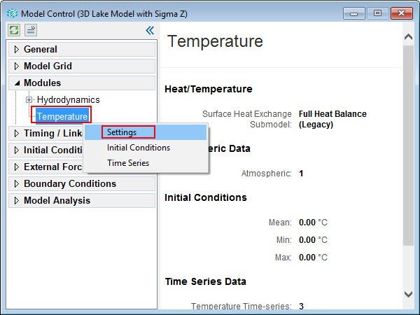
Figure 38. Open Temperature module.
- General tab
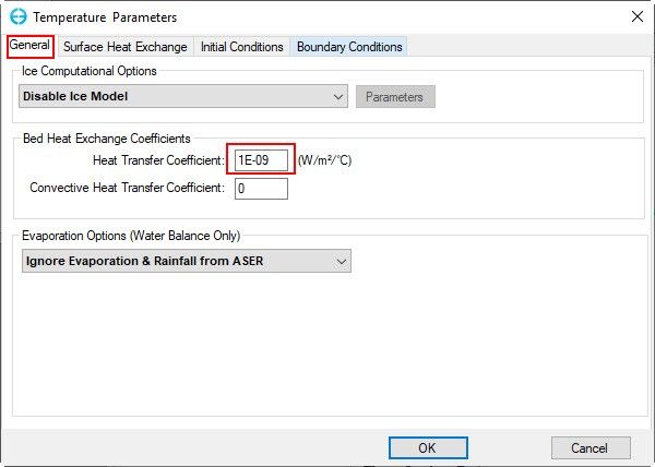
Figure 39. General Settings.
- Surface Heat Exchange
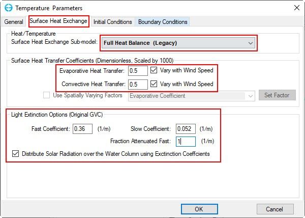
Figure 40. Surface Heat Exchange Settings.
- Initial Condition
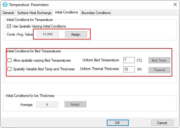
Figure 41. Initial Conditions Settings.
- Boundary Conditions
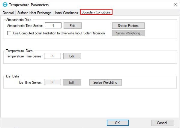
Figure 42. Boundary Conditions Settings.
7 Model Timing
After these, you are almost completed building the hydrodynamic model. This section will guide you on how to set up the model simulation time and model time steps.
- RMC on Timing tab in Timing/Linkage menu item to open the Simulation Timing Options form as shown in Figure 43.
- Enter values as shown in Figure 43. Note that the boundaries time series should be always cover this simulation duration period, otherwise the model will not run. The purpose of these settings is outlined in Table 2.
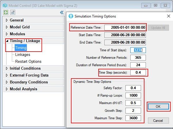
Figure 43. Model Run Time.
Table 2. Model Run Time Explanation.
Name | Explanation |
Time of Start (days) | Julian starting date (an automated conversion to Gregorian date is there) |
# Reference Periods | Total simulation time (an automated conversion to Gregorian date is there) |
Duration of Reference Period (hours) | Reference period |
Time Step (second) | Delta T |
Safety Factor | 0<Safety Factor < 1 to active the Dynamic time step |
# Ramp-Up Loops | Number of initial interaction to hold the time step to a constant during the ramp-up |
Maximum dH/dT | If >0 then it is an additional criterion to determine the dynamic time step. |
Beginning Date/Time | The base date of all data and simulation period. |
3. RMC on Linkage tab in Timing/Linkage section, the EFDC Model Linkages form will be displayed as shown in Figure 44.
Select the EFDC+ Explorer Linkage tab to set the Linkage Output Frequency. Setting this to 60 minutes means that EFDC will write the output every 60 minutes for displaying the model results in the EE (Figure 44). Note that a smaller output frequency will cause a larger output file. In this case, we will set the frequency equal to 30 min.
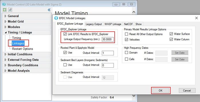
Figure 44. Setting Linkage Output Frequency.
8 Hydrodynamic Model Setup
This session will guide you on how to set the hydrodynamic model. The EFDC model applies a wetting and drying condition. Thus, we should set this condition as follows:
- RMC on Hydrodynamics menu item in Modules, and the Hydrodynamics Options form will be displayed as shown in Figure 46.
- Go to Wetting and Drying tab and set the as values shown in Figure 46 for optimizing in this case (note that wet depth should always greater than the dry depth).
- Save the model project.
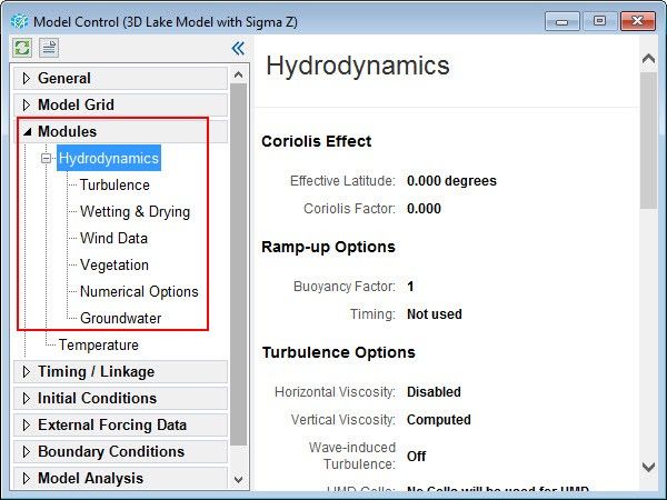
Figure 45. Open Hydrodynamics settings.
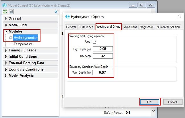
Figure 46. Hydrodynamic Options form.
9 Running EFDC
- Select the Run EFDC icon on the main form to open EFDC+ Run Options windows (Figure 47).
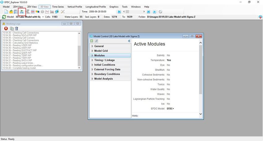
Figure 47. Open EFDC+ Run Options windows.
2. In this Window set the Number of OMP Threads to a number less than or equal to half the Max. Then browse to the EFDC Executable file (see Figure 48).
3. Click the Run EFDC+ button to run the model (Figure 48).
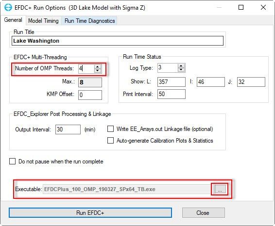
Figure 48. Run EFDC Settings.
If everything is set correctly, the model will start running and you will see the MS-DOS Window appear to display the model results as shown in Figure 49. Note that you can press any characters on the key-broad to pause the simulation and check the model results by using the Refresh button. If you want to exit the simulation select the same key, if you want to continue run then select any other key.
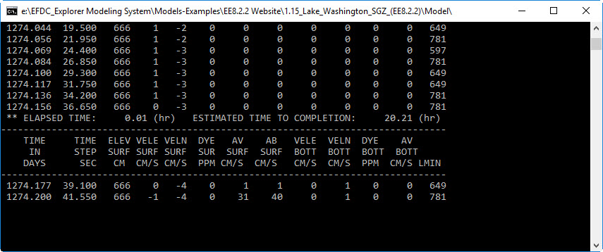
Figure 49 Running EFDC Window.
10 View the Model Calibration Plots
Go to Model Analysis Tab, select Model Calibration as shown in Figure 50. Click Define/Edit button to fill the Time Series Comparison form as shown in Figure 51 then click OK button to finish.
Then click the Plots button, a form for Calibration Plot Generation is displayed (Figure 52). If the user check on the two checkboxes, the EE will automatically generate plots and ASCII data file which are stored in #calib_plots folder. The user can stop the process by press the Escape button on the keyboard during automatic generation. Otherwise, the EE generates a plot one by one.
Time-series comparison and vertical profile comparison plots are shown in Figures 53 and 54.
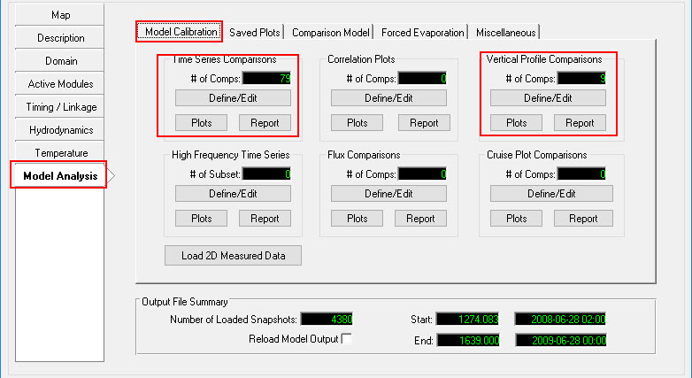
Figure 50. Model Calibration form.
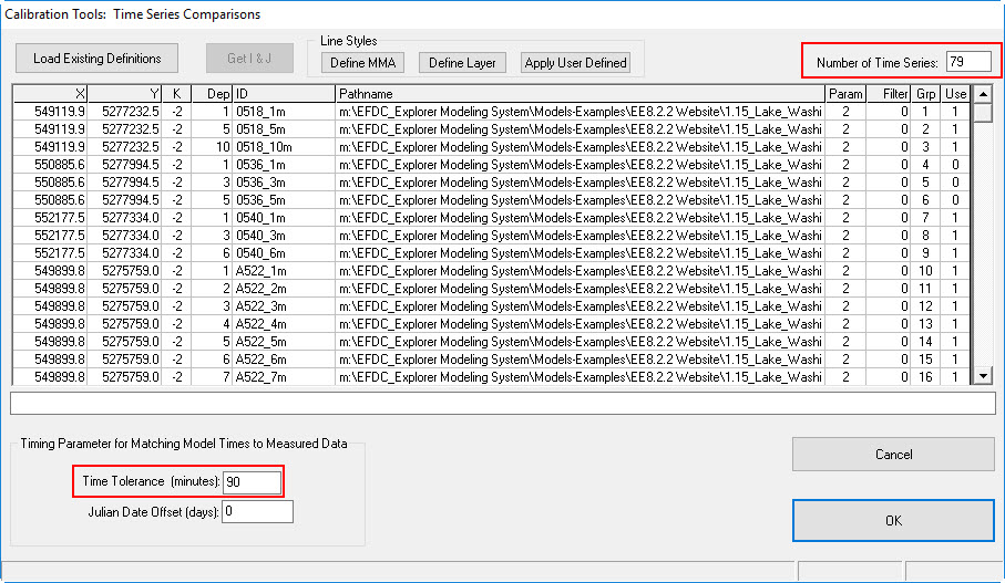
Figure 51. Time Series Comparisons form.
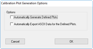
Figure 52. Calibration Plot Generation Options.
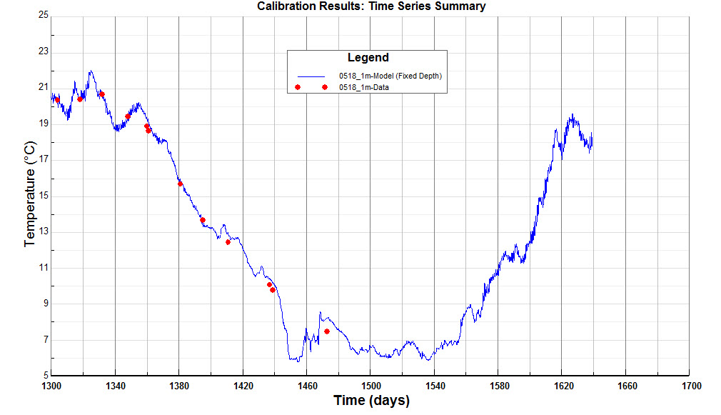
Figure 53. Time series comparison plot.

Figure 54. Vertical profile comparison plot.