The 2DH View window is shown in View Layer Control#Figure 1. The layers that are currently available to be displayed are shown in the Layer Control window on the left of the window. This layer control can be moved by user by dragging it with the cursor.
Clicking on icon  on the top-right of Layer Control frame gives a number of options as shown in View Layer Control#Figure 2.

Figure 1. View Layer Control in 2DH View.
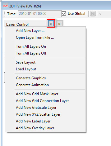
Figure 2. List of general options in View Layer Control.
- Add New Layer: allow to add more parameter layers from active model to 2DH View window. Details of this feature is described in Add a New Model Layer.
- Open Layer from File: this feature allows the user to open an external file with a range of data file formats such as *.p2d, *.shp, *.kml, *.kmz etc.
- Turn All Layers On: display all layers in 2DH View window, when this feature is selected all existing layers in Layer Control are displayed. Indication for this is all bulb symbols are lit (see View Layer Control#Figure 3).
- Turn All Layers Off: hide all layers in 2DH View window, when this feature is selected all existing layers in Layer Control are turned off. Indication for this is all bulb symbol are off (see View Layer Control#Figure 4).
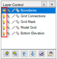
Figure 3. Light bulbs on when Turn All Layer On selected.
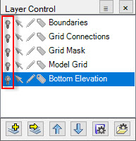
Figure 4. Light bulbs off when Turn All Layer Off selected.
- Save Layout: time frame, scale bar, north arrow, legend, layers etc that have been set in 2DH View, will be saved and can be loaded at another time without adjustment of the components. To save the layout, the user click on
 symbol of the Layer Control frame, the file 2DHView.2DL will be saved in the #analysis folder by default after clicking on the OK button. Another way to save the layout is go to 2DH View in main menu then select Save Layout (see View Layer Control#Figure 5 and View Layer Control#Figure 6).
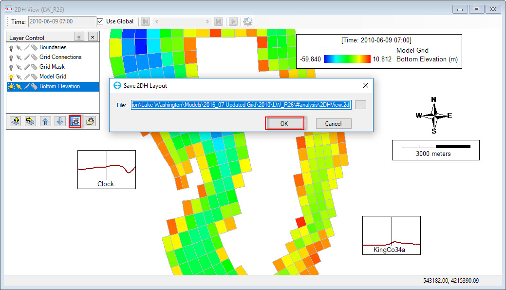
Figure 5. Save 2DH View layout (1).
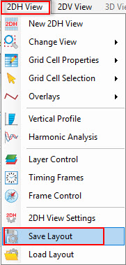
Figure 6. Save 2DH View layout (2).
- Load Layout: to load the layout which was saved in the past, click on
 symbol of the Layer Control frame or go to 2DH View in main menu then select Load Layout, browse to the file 2DHView.2DL, as default the file is in #analysis folder. If the saved layout also includes the layers, however the layer is not in the current view, the user should check the Load Layer Settings checkbox(see View Layer Control#Figure 7)
 - Generate Graphics: This is described in Export Images and Animations.
- Generate Animation: This is described in Export Images and Animations.
- Add New Grid Mask Layer: RMC to add masks as shown in View Layer Control#Figure 8.
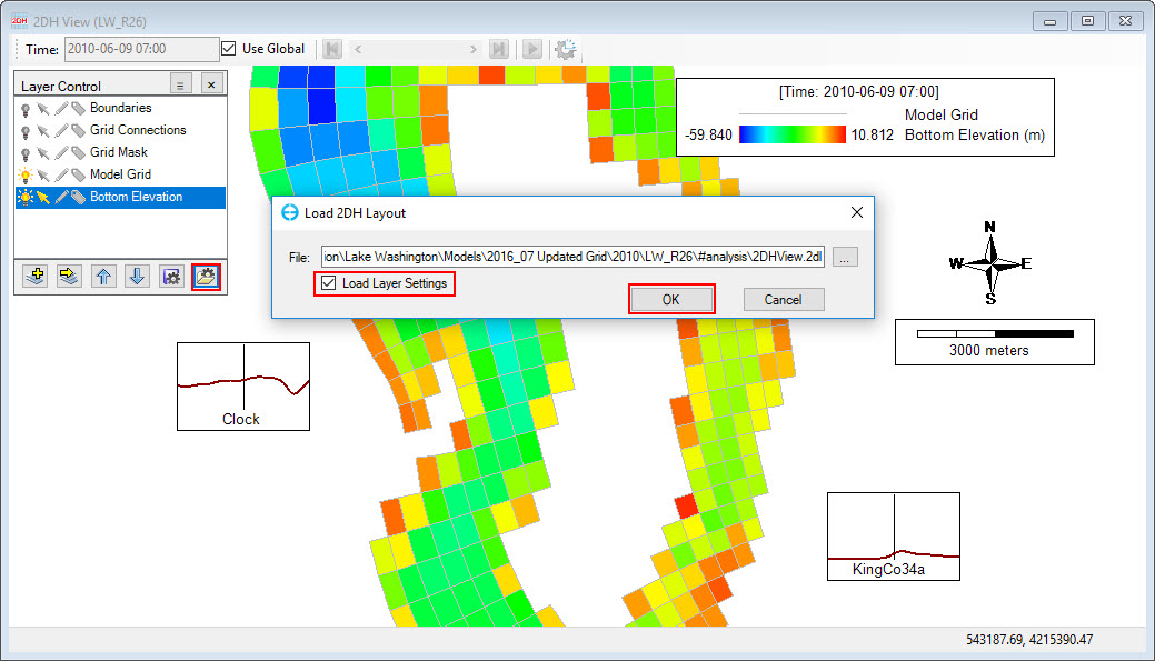
Figure 7. Load 2DH View layout.
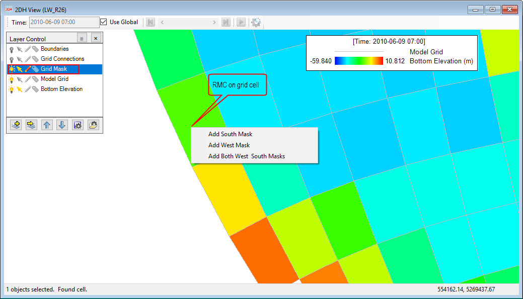
Figure 8. Add grid mask.
- Add New Grid Connection Layer: Add N-S or E-W grid connectors for different grid domains. Select Grid Connections layer in Layer Control then RMC on a cell from one grid which is to be connected to another grid, and select Add N-S Connection (or Add E-W Connection), then LMC to set the second connection point (see View Layer Control#Figure 9).
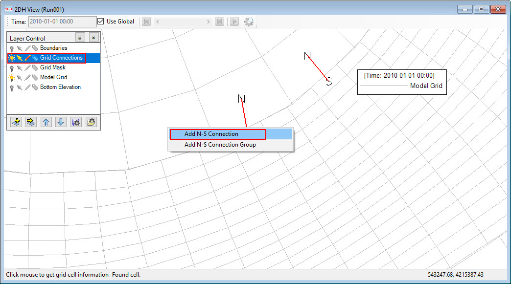
Figure 9. Add new grid connection.
- Add New Graticule Layer: this can be used to show the location in geographic coordinates (degrees latitude and longitude). RMC on the layer then select Properties, and the Graticule Settings form will be display. The user should customize the locations and interval of the lines as shown in View Layer Control#Figure 10 and View Layer Control#Figure 11. The graticule lines are displayed as shown in View Layer Control#Figure 12.
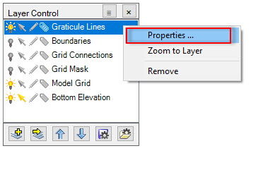
Figure 10. RMC on Graticule Lines Layer.
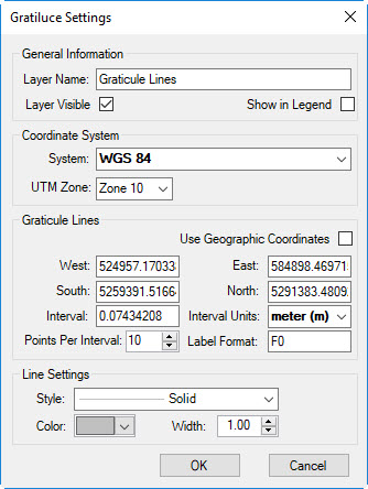
Figure 11. Graticule Settings Form.
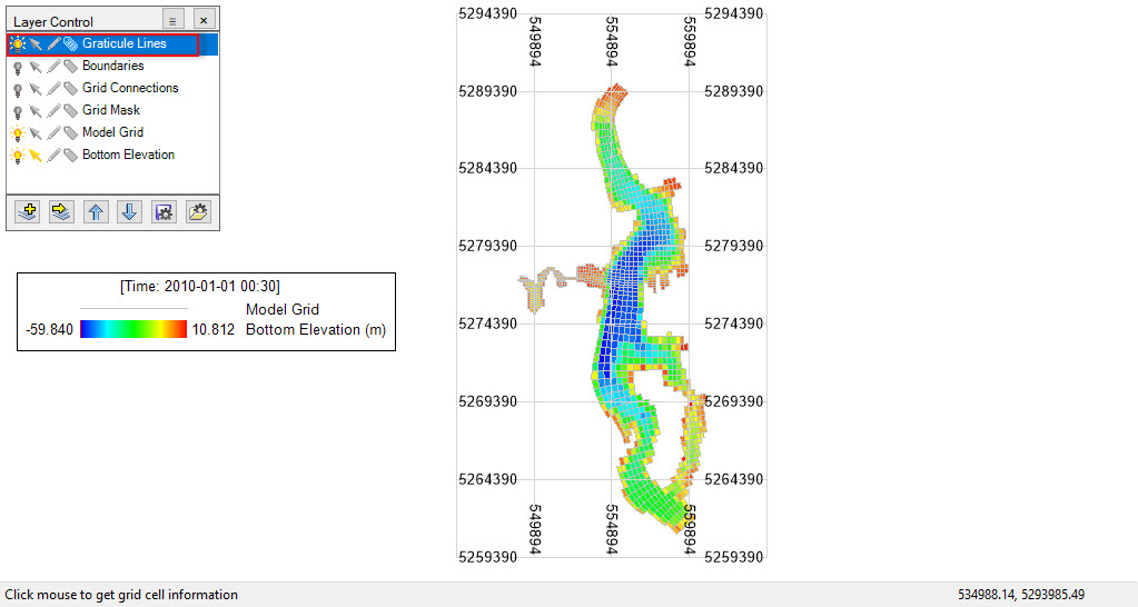
Figure 12. Graticule lines displayed in Layer Control.
- Add New XYZ Scatter Layer: when this option is selected an XYZ layer is added to the Layer Control. RMC on the 2DH View window then select Create New Data Point which displays the Data Point form, in which X and Y are coordinates in meters of each point, Z is the third field which could be elevation or concentration etc. The initial value of Z is zero and the user can edit this value by entering a new value. If the user wants to update new coordinates for the point then enter new values for X and Y (see View Layer Control#Figure 13). When RMC on the XYZ layer in Layer Control like Properties (set properties for data point), option include Export (save the XYZ file out), Remove (delete the layer) as seen in View Layer Control#Figure 14.
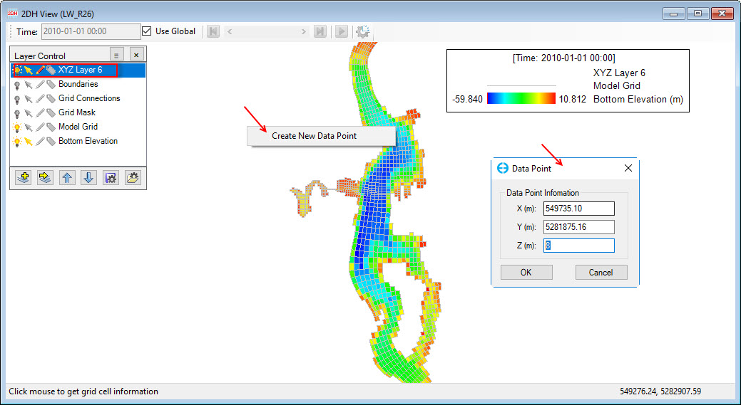
Figure 13. Add a data point to XYZ layer.
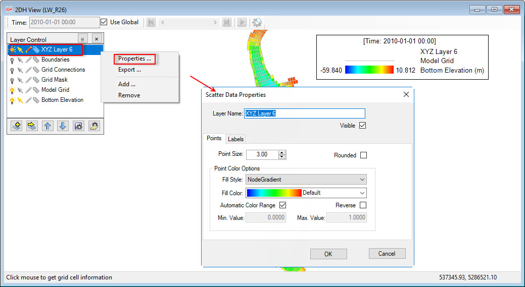
Figure 14. RMC options of the XYZ layer.
- Add New Label Layer: this allows to add a label layer, after this option is selected a label layer is added to the Layer Control. The user can RMC on 2DH View window then select Create New Label, a form of Label Properties appears, in which X and Y are coordinates in meters, Z is a third field containing information of the point such as elevation as shown in View Layer Control#Figure 15. The initial value of Z is 9999999.88 to make sure that the label is not covered by other layers. In this form, the user can change properties for labels such as name, symbol style, color, font etc. There are further options when RMC on the label layer in Layer Control including Properties (set properties for labels), Import (import a label file), Export (save the label file out), Remove (delete the layer from Layer Control). (see View Layer Control#Figure 16).
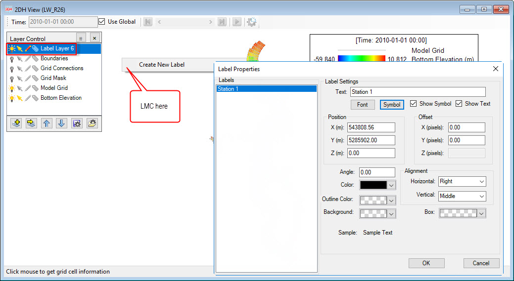
Figure 15. Add a label to Label Layer.
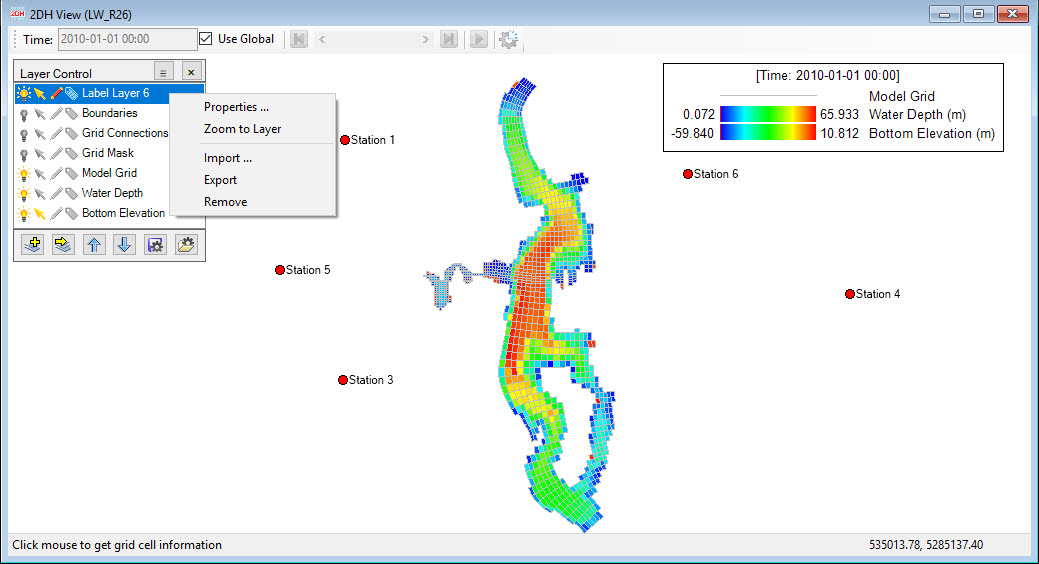
Figure 16. RMC options on Label Layer.
- Add New Overlay Layer: when this option is selected, a layer named Vector Layer is added to Layer Control. Note that the pencil symbol should be enabled. The user can then go to Poly Tools
 on the toolbar, select Draw Polyline and LMC on 2DH View window to start drawing a polyline. RMC to end drawing. RMC on the Vector Layer provides options such as Properties (set the properties for line and points of the polyline), Zoom to Layer, Save As and Remove. When the user selects Save As the Save As form appears, the user need enter a file name and file extension ( eg *.P2D, LDB, XYZ etc) then click Save button. As default the file is saved in #analysis folder as shown in View Layer Control#Figure 17, View Layer Control#Figure 18, and View Layer Control#Figure 19.
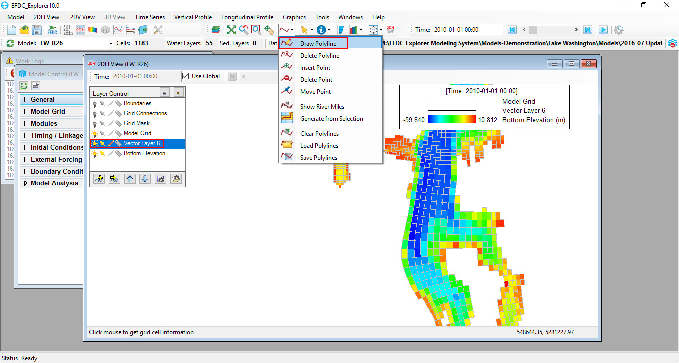
Figure 17. Add overlay layer.
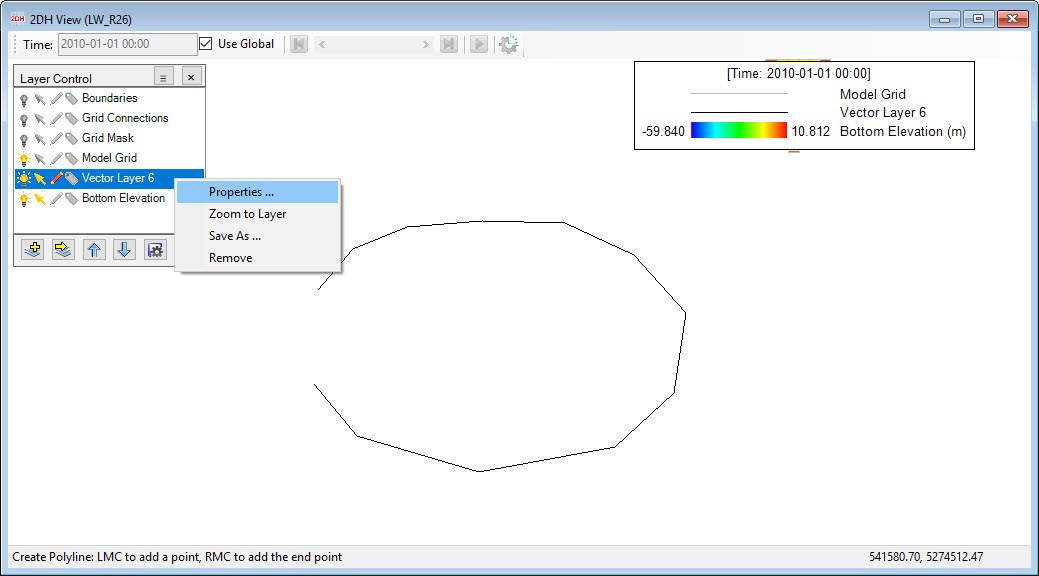
Figure 18. RMC Options of overlay layer.
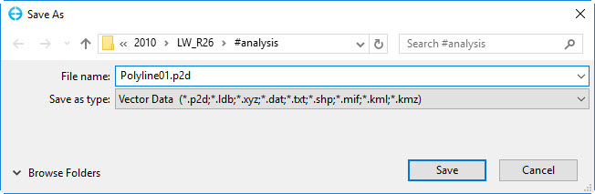
Figure 19. Save As overlay layer out.
When there are a number of layers in the Layer Control, the user might want to arrange order of the layers by selecting the layer first then using Up/Down arrows ( ).
).
There are four symbols accompanied with each layer: light bulb, arrow pointer, pen and label tag. Their meanings are described in View Layer Control#Figure 20.
RMC on layer in Layer Control, provides a number of options including Properties, Zoom to Layer, Edit, Export, Remove as shown in View Layer Control#Figure 21. These options can vary depending the type of layer selected. The Properties layer provides important options for configuring the layer viewing.
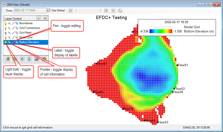
Figure 20. Function symbols of layer in Layer Control.
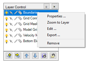
Figure 21. RMC on layer in Layer Control.