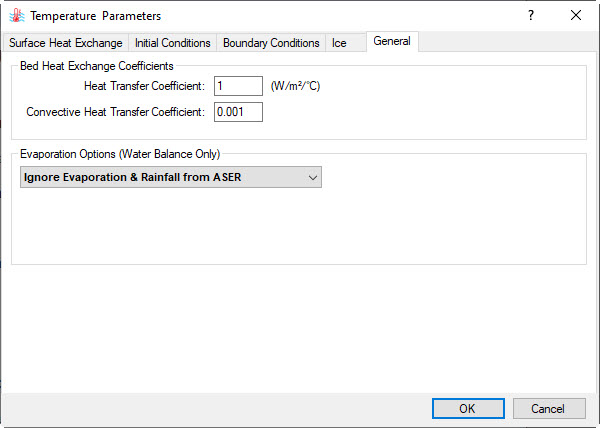
The General tab in the Temperature Parameters form allows the user to configure the Ice Computation Options, Bed Heat Exchange Coefficient, and Evaporation Options as shown in Figure 1. These options are each described in detail below. Note that by default the Display Options in EE are the water depth and water surface elevation include the ice thickness. This can be manually changed by the user in this option.
Anchor Figure 1 Figure 1
Figure 1. Temperature Parameters: General.
Ice Computation Options
A robust ice sub-model is available in EEMS. Older versions of EFDC had relatively limited ice modeling ability. Ice formation and melt is currently simulated by EFDC using a coupled heat model and fully handled by EFDC_Explorer.
Note that ice dynamics are not modeled at this stage. An ice dynamics sub-model would simulate the constriction of the channel by ice and the resulting bed shear caused by the transport of ice chunks. An ice dynamics sub-model is being considered for a later release of the EE modeling system.
Ice options are now available under the Ice Computational Options frame shown in Figure 2. For all these options, ice is only enabled if the user is simulating temperature.
...
Figure 2. Temperature Parameters: Ice Computation Options.
Options for the ice sub model include:
ISICE = 0 Disable Ice Model
ISICE = 1 Use External Ice Time Series (ISER & ICEMAP)
ISICE = 2 Use Specified ON/OFF Ice Cover
ISICE = 3 Use Heat Coupled Ice Model
ISICE = 4 Use Heat Coupled Ice Model with Frazil Transport
Application and operation of each of these options is explained in the following sections.
Use External Ice Time Series (ISICE = 1)
This option does not compute ice formation/melt and it is not linked to the heat balance. This option simply requires the user to provide a fraction of ice coverage and thickness of ice for every cell using formats provided in Appendix B - Data Formats. The primary impact of the ISICE =1 option is on processes that occur at the air/water interface and has no direct impact on ice melt. For those cells where ice is present the ice sub-model will:
- Limit water surface heat exchange and moderate the layer KC temperature to the specified ice temperature.
- Reduces or eliminates (based on fraction of ice coverage) re-aeration of oxygen into the water column.
- Reduces or eliminates the shear stress on the surface of the water due to winds.
- Reduces or eliminates the wind speed used for all other surface exchange processes.
...
Figure 3. Ice Parameters: ISICE =1.
Use Specified ON/OFF Ice Cover (ISICE = 2)
This option is effectively a global toggle so that ice may be turned on or off over the whole domain. The time series file that populates this option lists a date and toggle on and toggle off with the input file ISTAT.INP.
Figure 4. Ice Parameters: ISICE =2.
The input file ISTAT.INP file is same as old the ICECOVER.INP, with a time stamp and a status of ice cover. The convention is quite similar to that for other time series. The header contains the number of data lines, time conversion coefficients. The remaining block includes two columns: Julian time and the status of ice cover, either 0 or 1, off or on. The ice temperature and the ice thickness are stored in EFDC.INP file in C46A.
Appendix B shows the format for this file. EFDC reads the file and applies it in the same way as ICECOVER.INP. All the other computations are the same as those for ISICE=1 except the initialization is whole model on or off rather than based on the ICEMAP.INP file. EFDC can also handle multiple ice series and weights based on different series like NISER.
Use Heat Coupled Ice Model (ISICE = 3)
The Heat Coupled Ice Model applies mass conservation during ice growth/melt. Ice is always calculated in the heat coupled ice model, similar to CEQUAL-W2 model upon which the EFDC_DSI ice sub model is based. This option is most recommended for model simulations of lakes and reservoirs with relatively thick layers. For rivers, this option and frazil ice option are not fully representative. This is due to small layer thickness in most river models. Generally, the layers used in rivers are too thin to produce ice. Even though ice crystals form, they are not thick enough to form an ice cover.
Currently the ice sub-model in EFDC+is only an ice cover model and not an ice and snow cover model. The snow cover would account for snow on top of the ice and is expected to be added for an upcoming release. The ice cover model allows light to be attenuated through the ice. The solar radiation absorption is accounted for in this process. To implement this in EFDC, routines such as CALQVS and CALHEAT were modified. CALPUV was also updated so that the bed heat is handled when the elevation is below the bottom of the cell.
244023409 shows the default values of the ice parameters that are required to simulate ice in EFDC+ model. A checkbox is provided for the Use Ryan Harleman Wind Function option if desired.
...
Figure 5. Ice Parameters: ISICE =3.
ICE.INP is the initial conditions file that is only needed for ISICE = 3 & 4. The format for this file is provided in Appendix B. Note that EFDC assumes the top of ice is equal to the water surface elevation thereby allowing for higher flows in restricted depth.
Use Heat Coupled Ice Model with Frazil Ice Transport (ISICE = 4)
When calculating ice formation in a river, if the air temperature is less than freezing temperature (a value that may be lower than zero in salt water) generation of ice crystals takes place in the water. These crystals are called frazil flakes. As the frazil flakes are lighter than water they float and cause "ice pans" which may then become "ice floes". As the frazil ice rises, it is necessary to input a rising velocity into EE to account for this.
In addition to the modification to the EFDC subroutines outlined for ISICE =3, a new routine, CALTRANICE is created to simulate frazil ice as a concentration.
Figure 6. Ice Parameters: ISICE =4.
Visualization of Ice
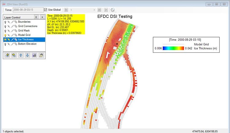
Output from the ice sub model can be displayed in a number of ways in EE. A 2D plan view of the ice thickness or temperature may be viewed by selecting 2DH View and then add layer Thermal/Ice | Ice Thickness. 244023409 shows an example of frazil ice formation in a river in Alberta, Canada. Note that initially ice forms on the river banks where depths are shallower and flow is lower.
...
Figure 7. Ice Sub model: 2DHView frazil ice thickness.
The user can also visualize ice on the water column in the 2DV View tool. This displays as a solid grey color as shown in Figure 8. The vertical exaggeration of the ice layer can be modified by RMC on Ice Thickness | Properties and change Thickness Factor to show it more clearly as shown in 244023409.
...
Figure 8. Ice Sub model: 2DV View ice cover and WC temperature.
...
.
Evaporation Options
The Evaporation Options (Water Balance Only) frame is only displayed if the appropriate surface heat exchange sub-model has been shown in the Surface Heat Exchange tab. Evaporation Options will only appear for the following surface heat exchange options:
...


