Activate the Temperature Module
The Graphical User Interface (GUI) for the Temperature module in EE can be activated from the EFDC+ Modules, as shown in Figure 1
Anchor Figure 1 Figure 1

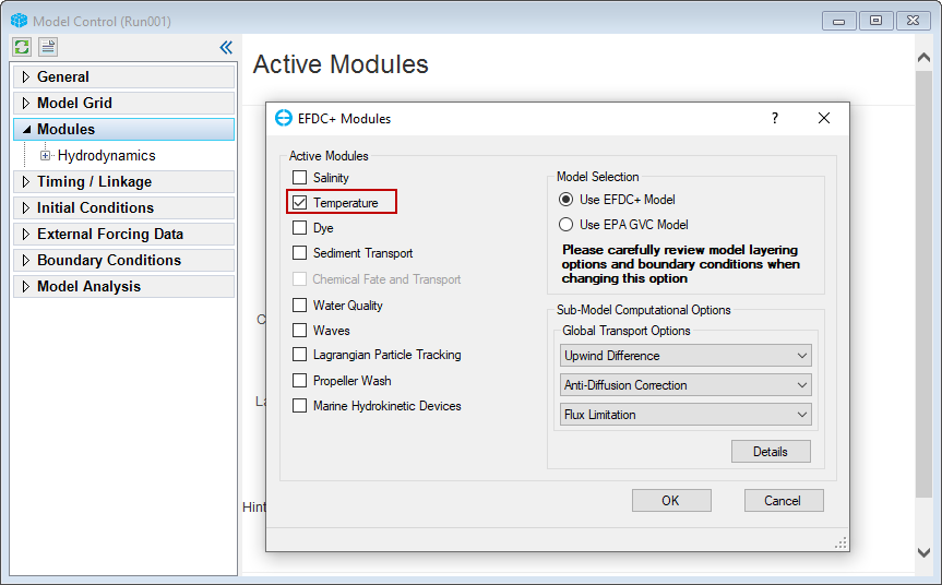
Figure 1. Active Temperature Modules.
Settings
After RMC on the Temperature module, the user can access the setting options, initial conditions options, or importing time data series Settings, Initial Conditions, and Time Series options (Figure 2).
Anchor Figure 2 Figure 2

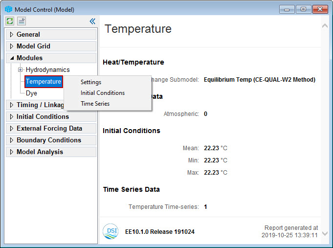
Figure 2. Model Control: Temperature ReportTemperature Module: RMC Options.
In order to set up the Temperature Module, the users should RMC Settings and then the Temperature Parameters form is displayed with five tabs. Each tab has different parameters that may be adjusted as described in the following sections (Figure 3).
| Anchor | ||||
|---|---|---|---|---|
|

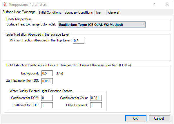
Figure 3. Temperature Parameters.
Initial Conditions
- Initial Conditions for Water Temperature: this can be set to a constant value or assigned to vary spatially. To set either of these options select the Assign button. To set a constant value simply enter a value in the Constant field under the Values to Set frame. The user can set this constant to certain layers in the Layer Options frame. If users want to use spatially varying initial temperature determined by a polygon, they should check the box and press The Apply Cell Properties via Polygons form is shown in Figure 5. If the values to be set vary spatially varying temperature based on XYZ or from vertical profile data, they should select one of these two options in the Values to Set frame. The user should then browse with the Add file button in the Data files frame to add these data sets. Various interpolation options are provided in the Interpolation Options frame, including replacement of existing data, and using the maximum or minimum values. Selecting the More button provides further interpolation options including order of inverse distance weighting (IDW) interpolation, number of neighboring points, and number of quadrants.
- Initial Conditions for Bed Temperature: It is able to set constant bed temperature by setting a value in the Uniform Bed Temperature box or check Use Spatially Variable Bed Temp and Thickness checkbox to assign a spatially varying initial temperature, by layer (Figure 6). The options and format of data files to upload to are described in Apply Cell Properties via Polygon. It also can select to apply cell properties for a specific layer or all layers in the model.
...
| Anchor | ||||
|---|---|---|---|---|
|
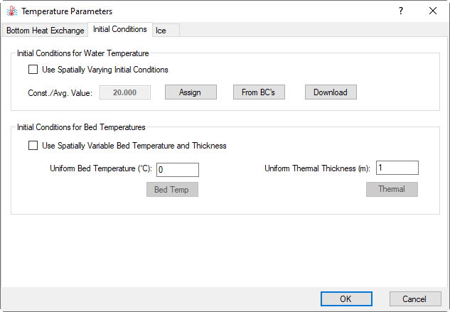
Figure 4. Initial Conditions - Temperature Parameters.
Anchor Figure 5 Figure 5

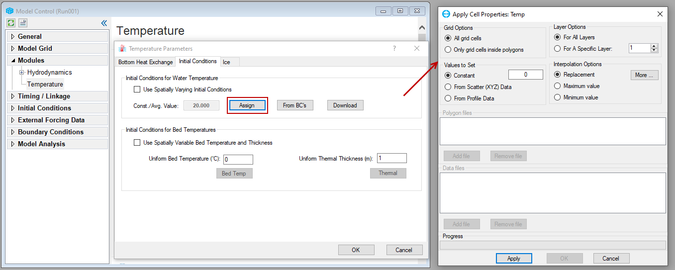
Figure 5. Assign Initial Conditions for Water Temperature.
Anchor Figure 6 Figure 6

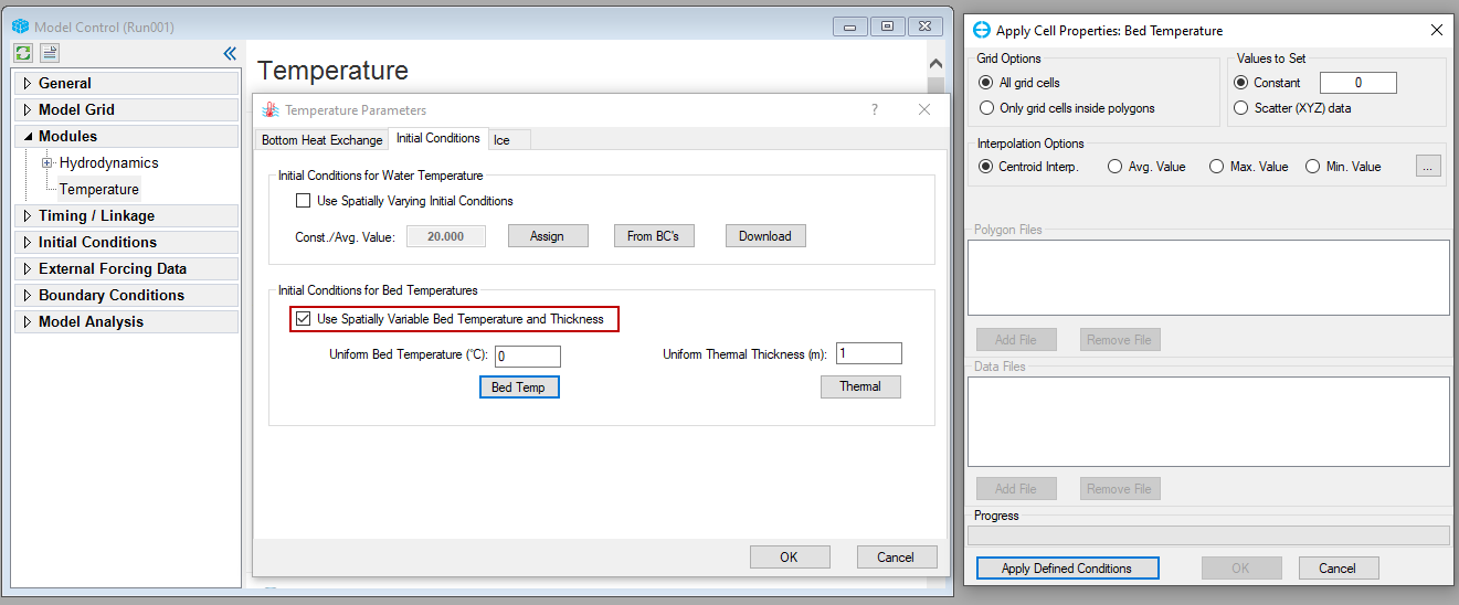
Figure 6. Assign Initial Conditions for Bed Temperature.
...
Visualization
2DHView2DH View
The temperature can be visualized and animated in 2DH View. These can be added to the 2DH View by clicking the Add button in the 2DH View’s Layer Control then select Primary Group: Water Column and Parameter: Temperature as shown in Figure 7
Anchor Figure 7 Figure 7

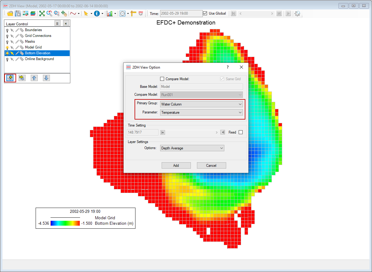
Figure 7. Temperature Layer in 2DH View.
Time Series
The graphic of temperature time series can be visualized by click the Time Series button or the icon ![]() of the main toolbar. The Extract Time Series Data tab appears as shown in Figure 8. It is possible to plot the time series for a single cell or multiple cells. Firstly, defying the cells to plots is in the box under Selected Cells. When the L index is entered the corresponding I and J indices are filled automatically. The parameter should be defined in the box, Primary Group: Water Column and Parameter: Temperature. Add and remove the parameter can be adjust adjusted by the left and right arrow button. The user may define the start and stop day for the time series in Time Series Start/Stop frame (note that the start and stop days should be within the model's start and end date). Clicking OK plots the selected graphs
of the main toolbar. The Extract Time Series Data tab appears as shown in Figure 8. It is possible to plot the time series for a single cell or multiple cells. Firstly, defying the cells to plots is in the box under Selected Cells. When the L index is entered the corresponding I and J indices are filled automatically. The parameter should be defined in the box, Primary Group: Water Column and Parameter: Temperature. Add and remove the parameter can be adjust adjusted by the left and right arrow button. The user may define the start and stop day for the time series in Time Series Start/Stop frame (note that the start and stop days should be within the model's start and end date). Clicking OK plots the selected graphs
Anchor Figure 8 Figure 8

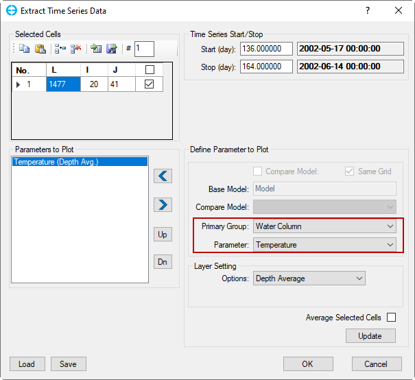
Figure 8. Extract Time Series Data.
Anchor Figure 9 Figure 9

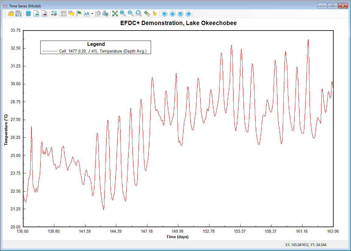
Figure 9. Temperature Time Series.
Vertical Profiles
The graphic of salinity vertical profiles can be visualized by click the Vertical Profile button or the icon ![]() of the main toolbar. The Vertical Profiles tab shows in Figure 10. It is possible to plot the vertical profiles for a single cell or multiple cells. Firstly, defying the cells to plots is in the box under Selected Cells. When the L index is entered the corresponding I and J indices are filled automatically. The parameter should be defined in the box, Primary Group: Water Column and Parameter: Temperature. Add and remove the parameter can be
of the main toolbar. The Vertical Profiles tab shows in Figure 10. It is possible to plot the vertical profiles for a single cell or multiple cells. Firstly, defying the cells to plots is in the box under Selected Cells. When the L index is entered the corresponding I and J indices are filled automatically. The parameter should be defined in the box, Primary Group: Water Column and Parameter: Temperature. Add and remove the parameter can be
...
adjusted by the left and right
...
arrows. It is possible to import an external file to compare with model results, that function is useful for the model calibration and validation.
Anchor Figure 10 Figure 10

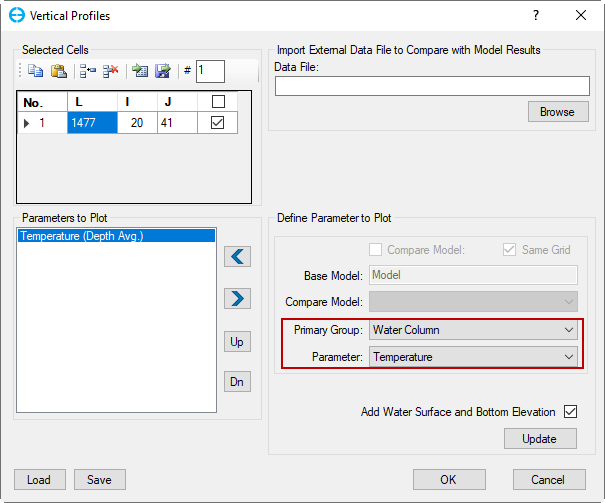
Figure 10. Vertical Profiles .
.
Anchor Figure 11 Figure 11
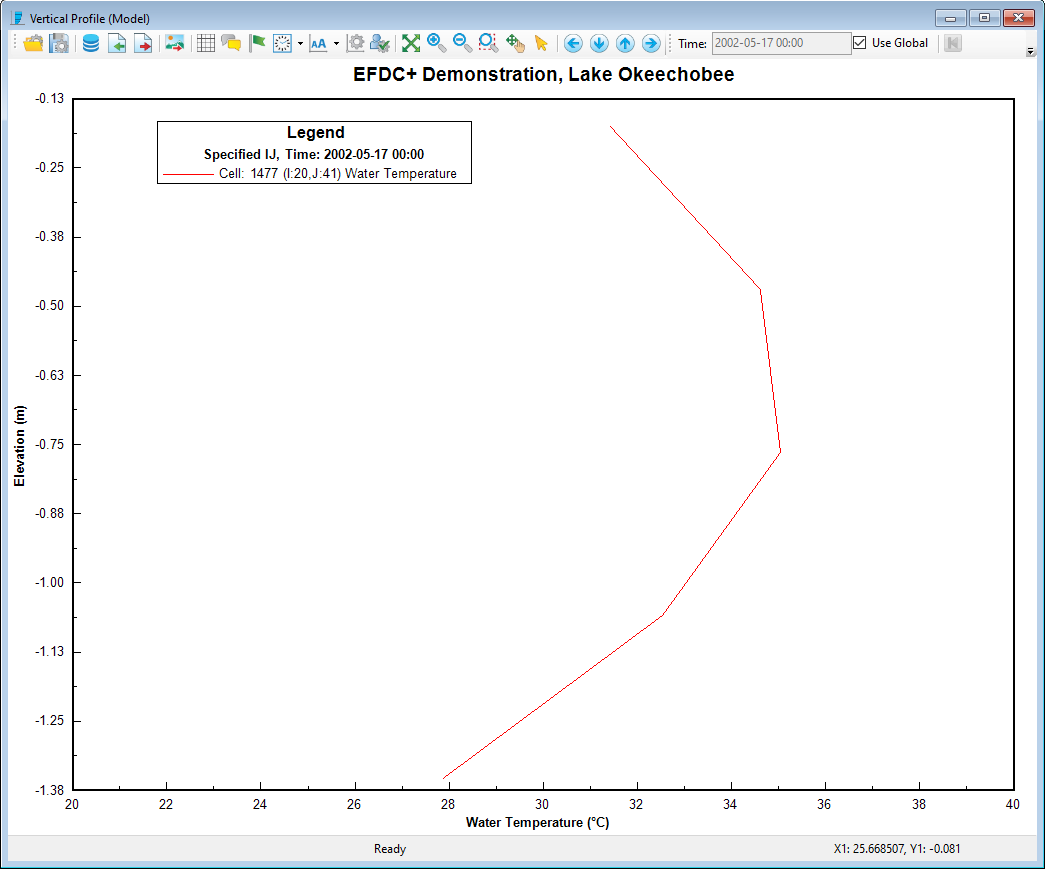
Figure 11. Water Temperature Vertical Profiles.
Longitudinal Profiles
The graphic of salinity longitudinal profiles can be visualized by click the Longitudinal Profile button or the icon ![]() of the main toolbar. Figure 12 show the Data Extraction for Longitudinal Profile form. This form is similar to the Data Extraction for 2DV View form. Firstly, it is necessary to define the profile using the drape file or I, J indices and then
of the main toolbar. Figure 12 show the Data Extraction for Longitudinal Profile form. This form is similar to the Data Extraction for 2DV View form. Firstly, it is necessary to define the profile using the drape file or I, J indices and then
...
define the parameter to the plot. Once everything is ready, click OK to generate the plot. Figure 13 shows a longitudinal profile for salinity and bottom elevation along with the profile I=39.
Anchor Figure 12 Figure 12

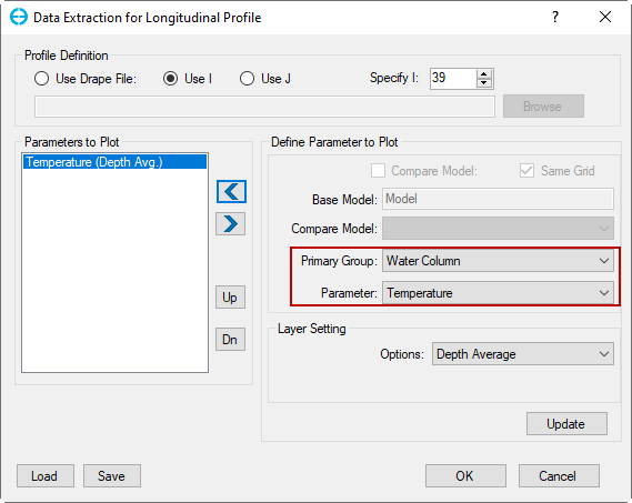
Figure 12. Data Extraction for Longitudinal Profile.
Anchor Figure 13 Figure 13

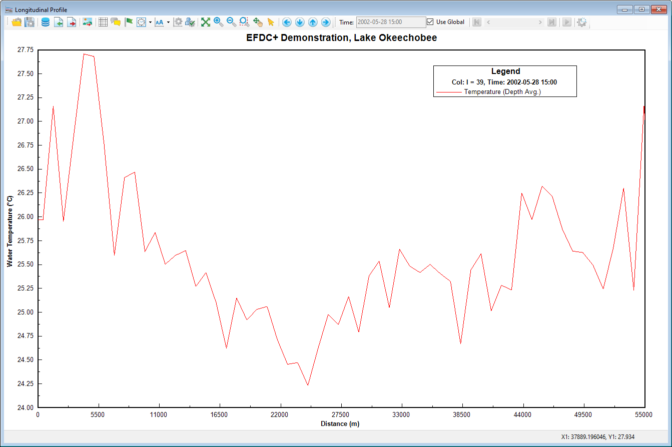
Figure 13. Water Temperature Longitudinal Profile.