1 Introduction
This tutorial will guide the user in how to set up a 2D lake hydrodynamic model and run a solution for EFDC. It will cover the preparation of the necessary input files for the EFDC model and visualization of the output by using the EFDC_Explorer (EE) Software.
The data used for this tutorial are from Hillsborough Water Atlas, Lake Thonotasassa, Florida, USA. All files for this tutorial are contained in the Demonstration Models of the Resources page folder file (DM-14_Lake_T_HYD-WQ_Model).
Before beginning the first session, let us first introduce the main form of the EE GUI in order to better understand our explanations in this document. Figure 1-1 is the main form of EFDC_Explorer or EE User Interface.
Figure 1-1. EFDC_Explorer main form.
2 Create a New Grid
This session will guide you to create a new simple grid with EFDC_Explorer.
Lake Thonotosassa is located in Hillsborough County, Florida, USA, and has been chosen as an example of where to build a 2D model in EE
The gird generation process includes the following steps:
1. Open EE
2. Click New Model icon:  on the main menu of the EE interface. The Cartesian Grid Generator frame appears shown in Figure 2-1
3. In Grid Options, select Uniform Grid.
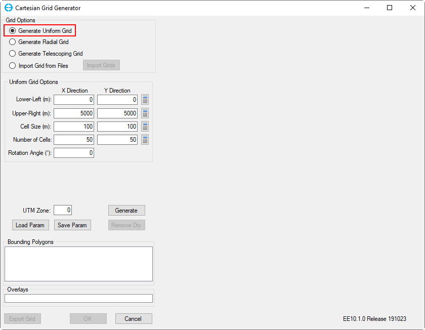
Figure 2-1. Generate EFDC Model form.
4. RMC (Right Mouse Click) on the Bounding Polygons blank to open a pop-up menu. In the pop-up menu, select Add Files to browse the polygon file. The land-boundary of the lake will be loaded here.
The polygon file for this model is "Outline.p2d" and can be found in Data/Bathymetry folder of the Demonstration Models provided above.
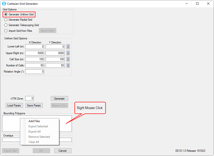
Figure 2-2. Add polygon file
5. With the polygon file loaded, the X-Y Directions for the corners of the models are automatically defined. The user can also adjust the Cell Size and Number of Cells in Uniform Grid Options.
In this example, enter cell size is 100x100m for the Cell Size (m) then click the calculator symbol for the Number of Cells.
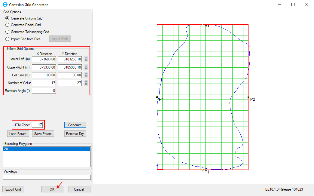
Figure 2-3. Loaded polygon file
6. If the user adjust any options in Uniform Grid Options they must click the Generate button so that EE can generate the changes.
7. Click on Remove Dry, this will remove all cells outside of the polygon.
8. Define UTM Zone for the model. In this case, the UTM Zone is 17 for Florida.
9. Click OK button to finish grid generation.
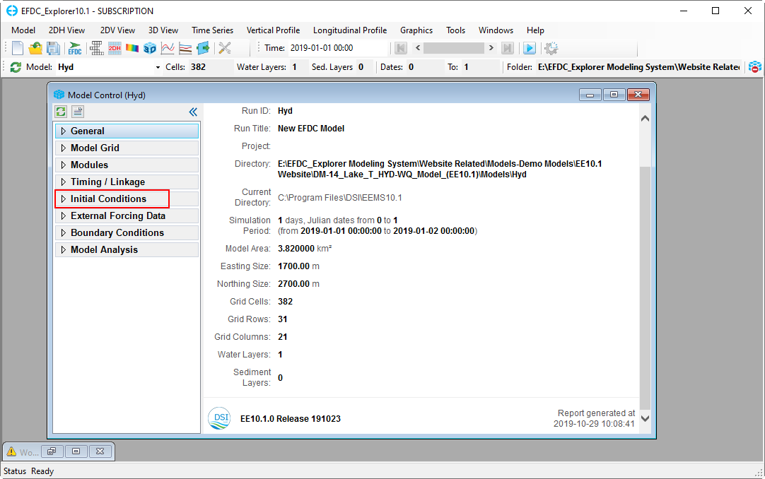
Figure 2-4. Grid information from generated model.
10. Save the model by selecting the Save button ![]() and create a new directory.
and create a new directory.
3 Assigning the Initial Conditions
This section will guide you on how to assign the initial conditions such as the bathymetry, water level, and bottom roughness.
Figure 3‑1. Assigning initial conditions.
3.1 Assigning the Initial Bathymetry
1. Select the Initial Conditions tab and right mouse click (RMC) on the Bathymetry sub-tab. A new Bathymetry form will appear. In that form, click on Assign to define bathymetric value.
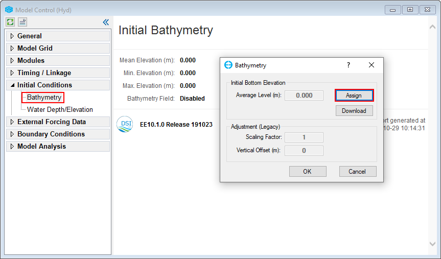
Figure 3‑2. Assigning bathymetry conditions.
2. The area the user wants to assign the bathymetry data to is set by a poly file. In this case, choose All grid cells
3. The data for bathymetry values are assigned by “Bathymetry.dat” file in Bathymetry folder . This bathymetry file is simply an xyz format.
4. Choose Scatter (XYZ) data and then Add file to browse for “Bathymetry.dat”.
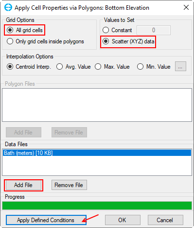
Figure 3‑3. Assigning bathymetry.
5. After adding the data file, click to the Apply Defined Conditions button to make your changes take effect before selecting the OK button.
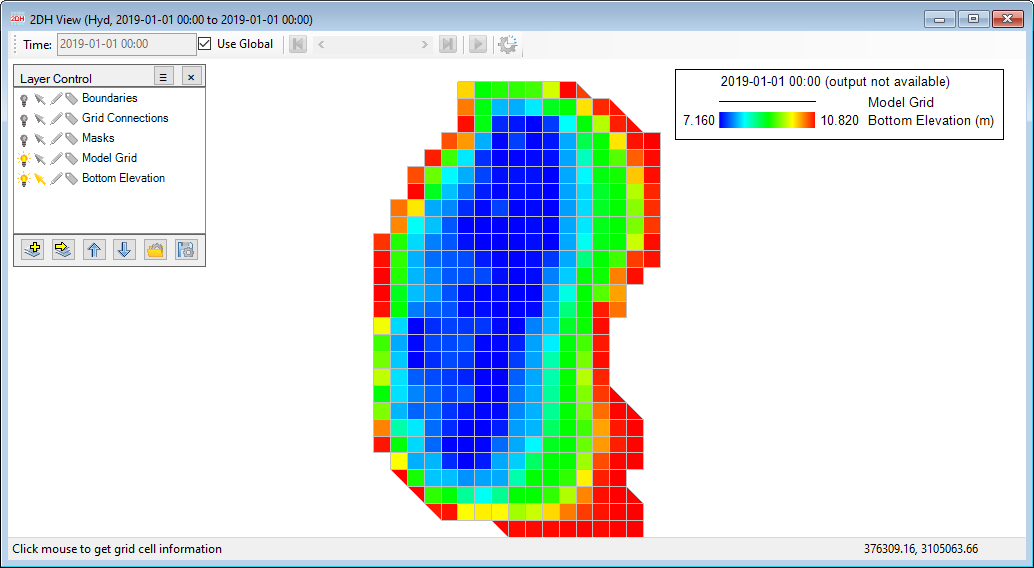
Figure 3‑4. 2DH View of bottom elevation after assigning bathymetry.
3.2 Assigning the Depth/Water Surface Elevations
This step assigns the initial depth or water surface elevations. There are two options for setting the surface water elevation, namely, use Constant and use Scatter (XYZ) data.
1. RMC on Water Depth/Elevation button then Click Assign Elevation button (Figure 3-5)
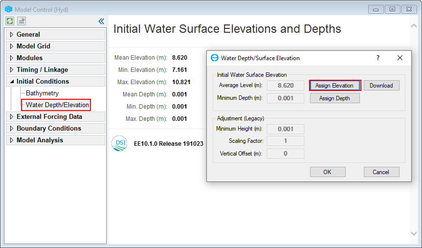
Figure 3‑5. Assigning water depth/surface elevation.
2. Select Constant to assign a constant water surface elevation of 11.5 m in the Constant box. (Figure 3‑6).
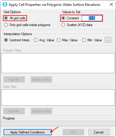
Figure 3‑6. Assigning water surface elevation (use constant option).
3. After selecting this option for assigning water surface elevation, click Apply Defined Conditions button then click the OK button to finish.
4 Boundary Conditions
This section will teach you how to prepare the boundary conditions and assign them to the model cell configuration. In this Lake 2D case there are two flow boundaries; one is runoff inflow to the lake and the other is outflow through a gate. Thus, we should prepare two time series of inflow and outflow boundaries. In other cases, the number of time series for boundary conditions might be much more such as those for hydraulic structures, pressure boundaries, or include time series for temperature, salinity, and water quality boundaries also.
4.1 Set Time Series
To set the boundary time series take the following steps:
1. Select the External Forcing Data tab. (Figure 4‑1)
2. RMC on Flow button and select Add New Data Series to edit the flow boundary. (Figure 4‑1)
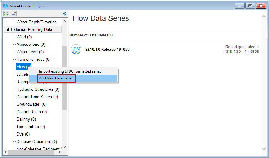
Figure 4‑1. Create flow time series.
3. Enter the Number of Series into the box. There are two flow boundaries as mentioned so it should be “2”.
4. Give a Series Name for associated time series. In this case, title “Inflow” for Series 1, and “Outflow” for Series 2. (remember to press Enter after each input)
5. Copy and Paste time-series data, “Inflow.dat” into the workspace corresponding to the Inflow series. Figure 4‑2 shows the time series of inflow.
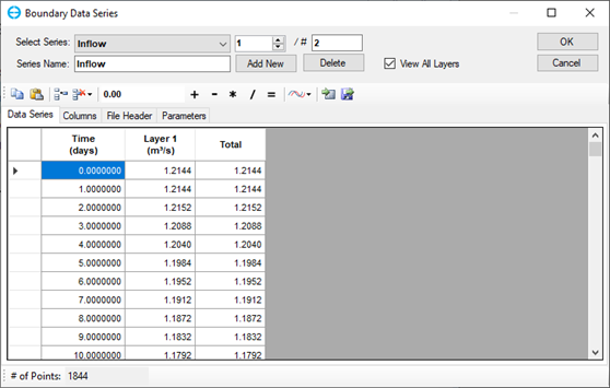
Figure 4‑2. Data series: Inflow.
6. Click to the View Time series plot icon to view the current time series (for a case where there are multiple layers check Sum Layers to show total flow).
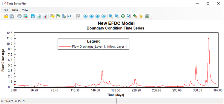
Figure 4‑3. Time series plot of inflow.
7. Select the up/down arrow buttons to edit the other time series.
8. Copy and paste time series data of outflow from the “Outflow.dat" in Boundaries folder into the workspace corresponding to Outflow as shown in Figure 4‑4. The time series plot of outflow is shown in Figure 4-5.
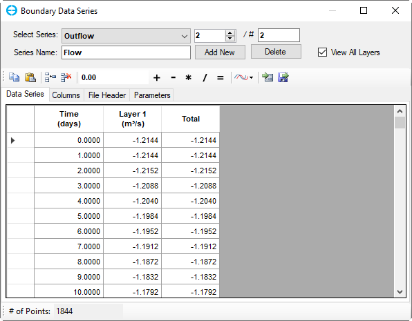
Figure 4‑4. Data series: outflow.
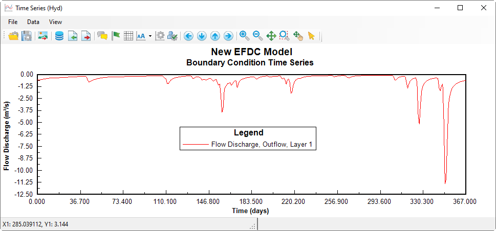
Figure 4‑5. Time series plot of outflow.
9. Click OK to finish editing the boundary time series.
After completing the above steps, the user has prepared all the required boundary time series. Now we will assign these boundary time series to the model cells. Figure 4‑6 shows the location of inflow and outflow for this lake case. Thus, we have to assign these cells with associated time series for in/outflow prepared in the previous session.
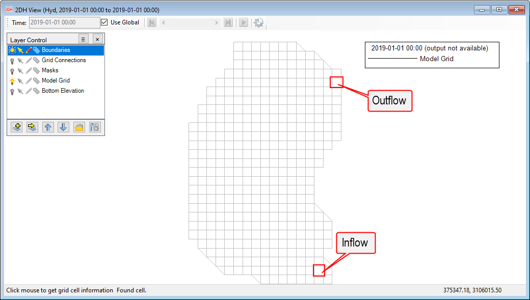
Figure 4‑6. Locations of inflow and outflow for the lake.
4.2 Assigning a Boundary Condition
In order to assign the boundary, the following steps should be taken;
1. Click the 2DH View icon ![]() on the main form of EE (Figure 1‑1).
on the main form of EE (Figure 1‑1).
2. Choose Boundaries in the Viewing Layer Control .
3. Enable Edit grid by turn on the icon ![]() (see Figure 4‑7)
(see Figure 4‑7)
4. RMC on the inflow location cell and select Add New Boundary Group (Figure 4‑8)
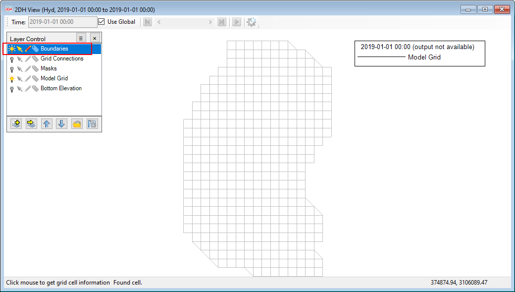
Figure 4‑7. Enable to edit Boundaries layer.
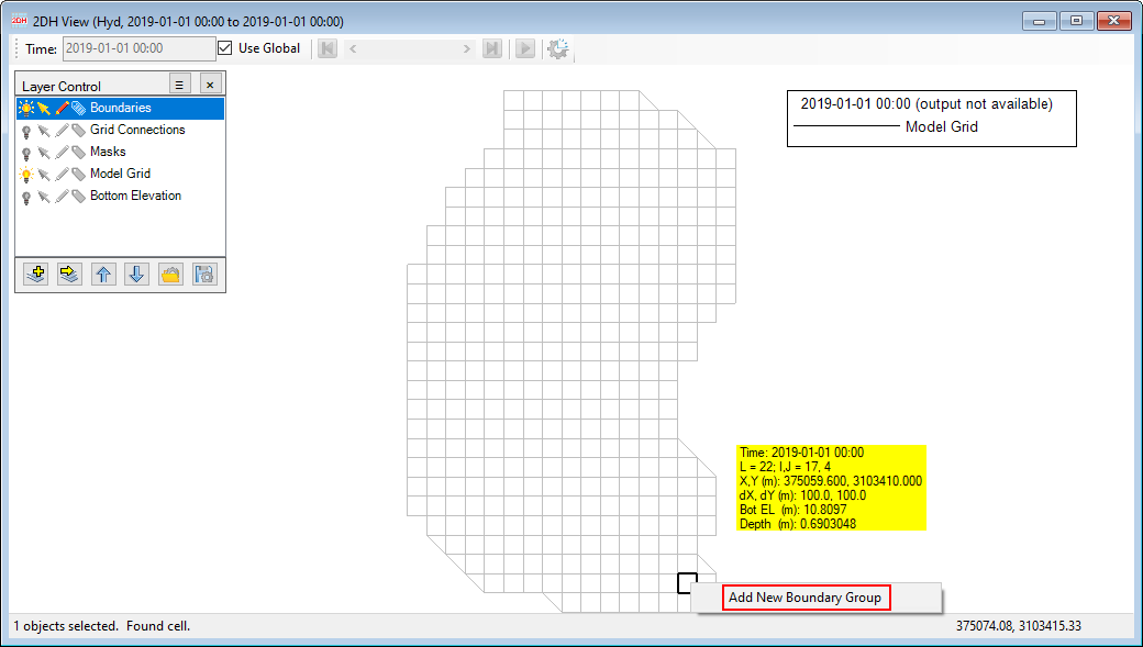
Figure 4‑8. RMC on the inflow cell to add a boundary condition.
5. Enter the Boundary Group Name by typing “Inflow” and select boundary types (Figure 4‑9). Then click OK button, the Flow Boundary Conditions form appears, in the Forcing Assignment frame, select "Inflow" for Flow Table (Figure 4-10), then click OK button.
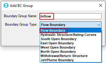
Figure 4‑9. Enter Boundary Group Name and select Boundary Group Type.
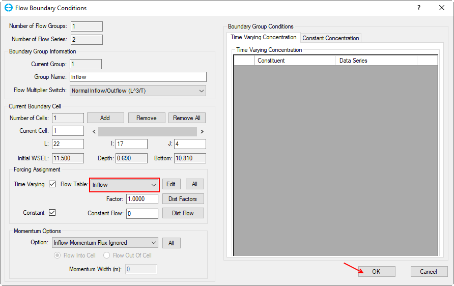
Figure 4‑10. Assign the corresponding time series.
If there are more than one Boundary Cells, the user must click on All to select all boundary cells then click on Dist Factors to distribute the factor to all boundary cells. The sum of Factor for all boundary cells must equal 1.
6. Apply the same process for assigning the outflow boundary cell. Figure 4‑11 presents the boundary conditions after assigning the inflow and outflow boundaries.
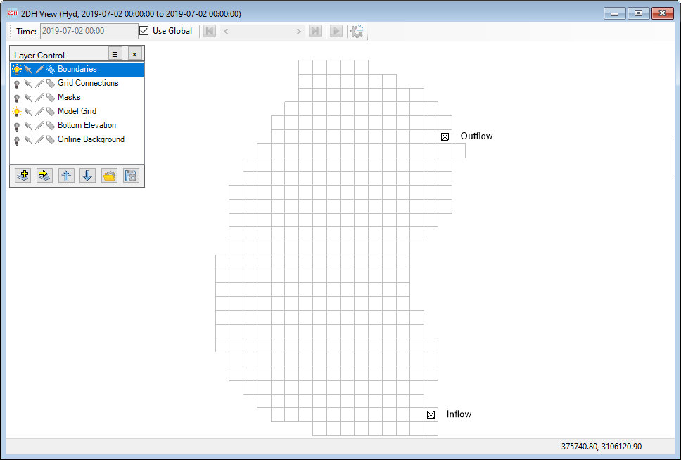
Figure 4‑11. Inflow and Outflow boundaries assigned.
5 Model Timing
After completing the previous sections, the user has almost completed the hydrodynamic model of a lake. This section will guide the user on how to set up the model simulation time and model time steps.
1. Select Timing/ Linkage tab and RMC on Timing button (Figure 5‑1)
2. Enter the duration of start/ end of the simulation. Note that the boundaries time series should always cover this simulation duration period, otherwise the model will not run.
3. Enter the Time of Start, Number of Reference Periods, Duration of Reference Periods and Time Step as Figure 5-1. These values are explained in Table 2 of Build a 2D Lake Model with EE8.
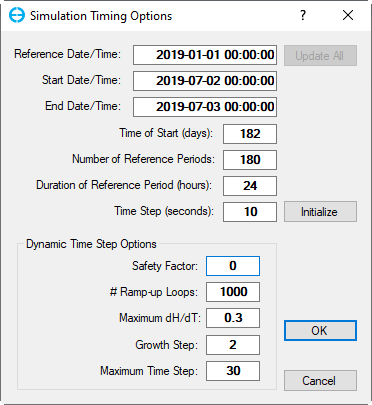
Figure 5‑1. Model run time.
4. RMC on Linkage button and set Link EFDC Results to EFDC_Explorer and set Linkage Output Frequency to 60 minutes. This means that EFDC will record the output every 60 minutes for the display of the model results in the EE. (Figure 5‑2). Note that a smaller output frequency will create a larger output file.
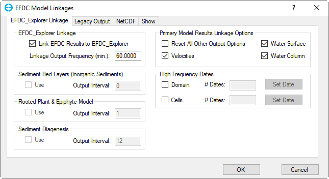
Figure 5‑2. Setting linkage output frequency.
6 Hydrodynamic Model Setup
This section will guide the user on how to set the hydrodynamic model for the EFDC model’s application of the wet and dry conditions to optimize the simulation time. For this condition we should make the following settings:
1. Select Modules tab then LMC on plus sign ![]() of Hydrodynamics to expand all sub-tabs. RMC on each sub-tab to adjust settings.
of Hydrodynamics to expand all sub-tabs. RMC on each sub-tab to adjust settings.
2. Select Shallow Water then RMC, the form of Shallow Water Options appears
3. Enter values for the Dry Depth and the Wet Depth. Then click OK button. Note that the wet depth should always greater than the dry depth. (Figure 6‑1).
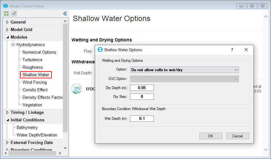
Figure 6‑1. Hydrodynamic model setup.
4. Return to select Model Grid tab, RMC on Grid sub-tab and enter the number of vertical layers required into the box. In this case, we will set the vertical layers equal to 5 (Figure 6‑2). Click OK button.
5. Save the model.
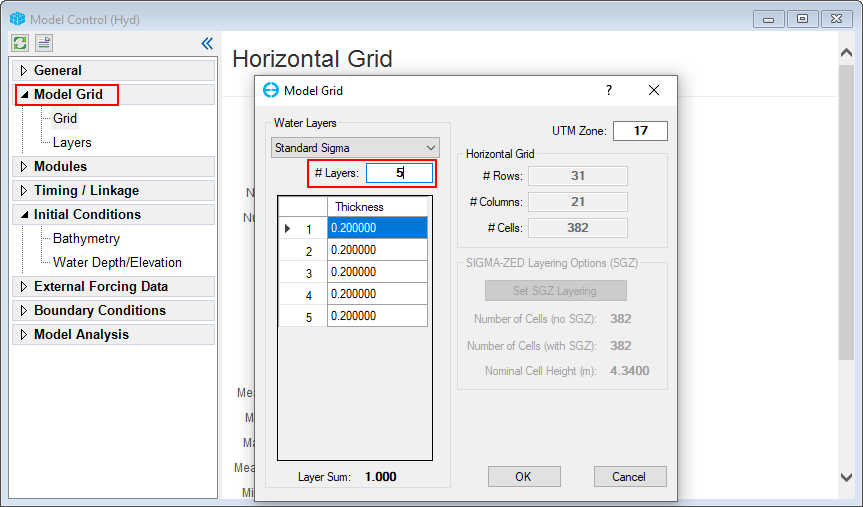
Figure 6‑2. Setting the vertical layers
7 Running EFDC+
This section runs the EFDC model and includes the following steps:
1. Click the Run EFDC icon ![]() on the main form
on the main form
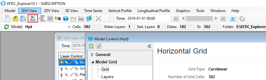
Figure 7‑1. Run EFDC+.
2. Select the Browse icon next to the Executable text box to browse to the EFDC executable file (Figure 7‑2) as default the EFDC+ executable file is located in the EEMS installation folder (e.g C:\Program Files\DSI\EEMS10.3)
3. To save time when running the model, the user can increase the number of OMP threads.
3. Click the Run EFDC+ button to run the model (Figure 7‑2).
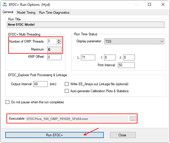
Figure 7‑2. Browse to the EFDC+ executable file.
If all settings are correct, the model will start running and you will see the MS-DOS Window appear showing the model results as shown in Figure 7‑3
Note that you can press any characters on the keyboard to pause the simulation and check the model results. If you want to exit the simulation hit the same key again, if you want to continue run then hit any other key.
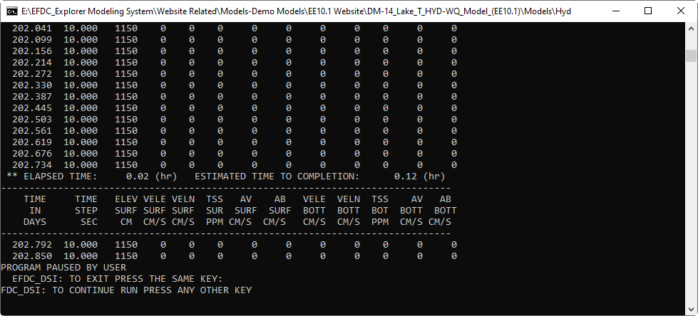
Figure 7‑3. EFDC+ run window.
Note that the user needs to click on the Refresh Model Output button  to allow EE to read, updates, and visualizes model output after finish running EFDC+.
8 Visualizing the EFDC Model Output
This session will teach you how to view the model simulation results. In general, selecting these three icons  on EE’s main form (Figure 1‑1) to view the model simulation results in 2DH View, 2DV View or 3D View, respectively.
1. Select the 2DH View icon
2. In View Layer Control, select Add a New EFDC View Layer (Figure 8-1). The user should see View Options window with Primary Group and Parameter to display.
3. Figure 8‑2 is an example of showing the vector and magnitude velocity field results. Similarly, the user can select other parameters to show the model results.
4. Right mouse-click on the Velocity vector layer to modify vector arrow sample or change vector color and scale factor (See Figure 8-2)
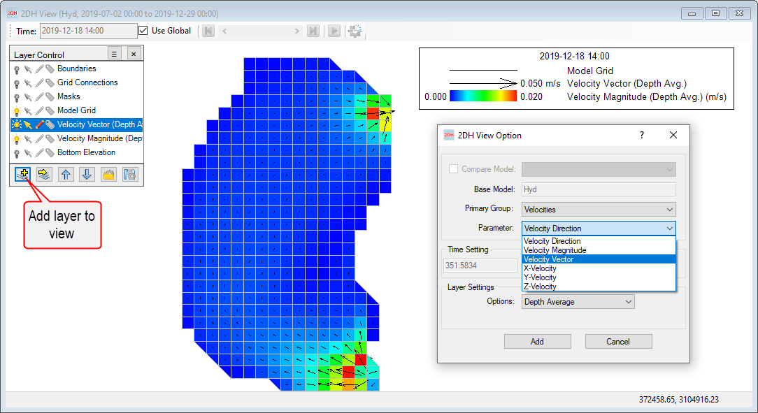
Figure 8‑1. View Layer Control and View Options.
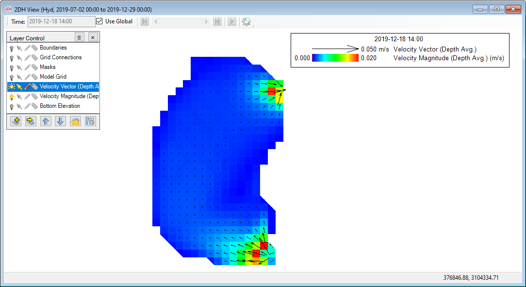
Figure 8‑2. Visualizing the EFDC model output.