The Habitat Suitability Criteria (HSC) models provide an objective, quantifiable method of assessing the existing habitat conditions for a given aquatic species within a study area by measuring how well each habitat variable meets the habitat requirements of the species by life stage. This serves as an objective basis for predicting probable project impacts, documenting post-project impacts, and guiding habitat protection, mitigation, enhancement, and management decision.
Instream Flow Incremental Method (IFIM) is a method of determining the HSC, and is one of the most widely used instruments in the world for assessing the effect of flow manipulation on river habitats. Originally developed by the US Fish and Wildlife Service (Bovee, 1982), USA EPA describes IFIM as integrating “concepts of water-supply planning, analytical hydraulic engineering models, and empirically derived habitat-versus-flow functions to address water-use and instream-flow issues and questions concerning life-stage-specific effects on selected species and the general well-being of aquatic biological populations. The method has undergone continual refinement by the Fort Collins Science Center scientists and has remained a state-of-the-art tool. A major component of IFIM is a collection of computer models called the Physical Habitat Simulation Model (PHABSIM). This model incorporates hydrology, stream morphology, and microhabitat preferences to determine relations between streamflow and habitat availability” (EPA, 2018).
At this stage, however, the PHABSIM models to not simulate water quality. PHABSIM concentrates on simulation of physical habitat based on depth, velocity, and a channel index. In their manual on PHABSIM, Milhous and Waddle (2012) refer users to other sets of models, such as the QUAL-2 model for approaches to simulate water quality constituents. Furthermore, PHABSIM, River2D and similar IFIM models are restricted to 2D simulation. With EEMS now enhanced to perform the IFIM analysis, it serves as a fully highly advanced 3D PHABSIM, incorporating water quality, sediment, toxics and many other highly relevant sub-models.
Habitat availability with IFIM is measured using an index called the weighted useable area (WUA). This is the wetted area of a stream weighted by its suitability for use by an organism. In EE WUA is calculated using the product of the habitat suitability indices, which are further described below:
|
|
Where
AL is the area of the cell
CL is the habitat suitability index for the channel index associated with the cell substrate and/or vegetation, if not used or needed a value of 1.0 is used,
L is the cell index
Si is the habitat suitability index for parameter i for up to n parameters.
Another common measure is weighted usable volume (WUV),
|
|
Where
VL is the volume of the cell
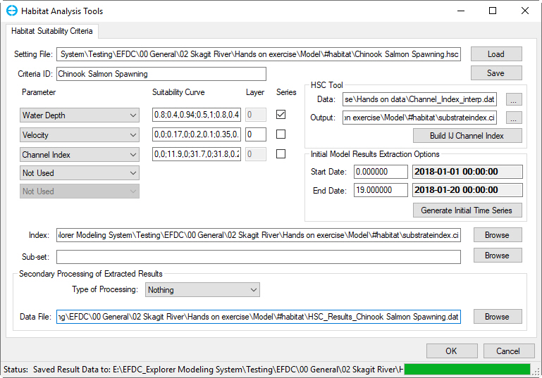
The interface for the IFIM approach to configuring habitat suitability criteria in EE is shown in Figure 1. When saving and loading the configuration files for habitat suitability criteria, EE uses “.HSC” as the file extension and it's directory path will be displayed in Setting File box
The Criteria ID will be used to manage the different species. The Criteria ID is appended to the file name “HSC_Results” of the data file extracted when generating an initial time series. For the example shown in Figure 1 the extracted file will be called “HSC_Results_Chinook Salmon Spawning.dat”.
Figure 1 Model Analysis: Habitat Suitability Criteria form.
Parameters that may be defined include bottom elevation, water depth, bed shear, channel index, velocity, fraction of light, cohesives, and TSS. The general approach for calculating the weighted usable area (WUA) for habitat is quite similar to that for the critical limits approach. One significant difference in the model setup is that the inflows are incremental, or stepped in IFIM approach. There are two main differences in the post-processing of the data: defining suitability index curves, and specifying a channel index. These are described below.
Suitability Index Curves
Rather than using simple maximum and minimum limits for a parameter, as was the case for critical limits, the HSI approach uses Suitability Index (SI) curves. These SI curves are constructed by quantifying field and laboratory information on the effect of each habitat variable, such as temperature, dissolved oxygen, spawning gravel size, and siltation, on the growth, survival, or biomass of a species by life stage. The SI curves assume that increments of growth, survival, or biomass plotted on the y-axis can be directly converted into an index of suitability on the x-axis. The index of suitability ranges from 0.0 to 1.0 with 0.0 indicating unsuitable conditions and 1.0 optimal conditions. Measurements of each habitat variable taken at the proper time in the field can be applied to the SI curves to assess the suitability of the variable in meeting the habitat requirements of the species by life stage
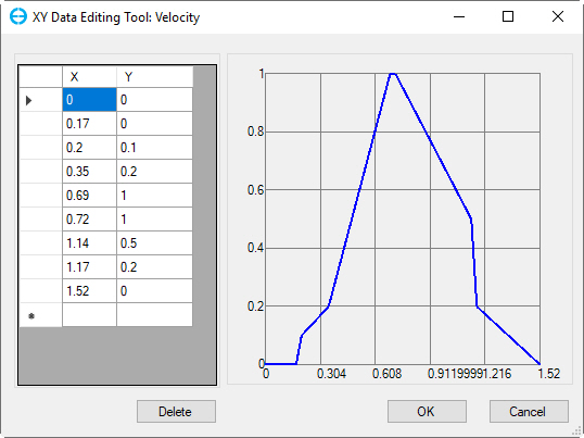
To facilitate the input of these curves, EE provides a tool to create and view SI curves. After selecting a parameter from the dropdown menu, selecting the Suitability Curves text box and pressing Enter will open the XY Data Editing Tool, which is a spreadsheet type form with a corresponding graph as shown in Figure 2. The user may choose to initially develop the curves in a spreadsheet and copy them into the Suitability Curve form where they will be stored and plotted. Alternatively, they can be typed directly into the form as (parameter, suitability). These x, y values are comma delimited, with each pair then separated by a semi-colon.
After defining the SI curves the user should select the layer range as described in the Critical Limits section. It is required to select the checkbox to assign which series is to be plotted, and the start and end date of extraction from the model, before selecting Generate Initial Time Series.
Figure 2 Editing tool for suitability index curves.
Channel Index
Another option available in the HSC approach, which is not in the Critical Limits option, is the defining of a channel index. The purpose of the channel index is to allow the user to evaluate the habitat suitability based on nature of the channel bed, which may vary in different regions of the stream, for example with sand, silt or gravel. This index can be set based on different locations in the channel that the species may be occupying. The channel index is a numeric value that has been assigned to each cell. EE allows the user to assign any value to a cell, though typically they range from 0 to 1, or 0 to 100. Channel index is one of the parameter options, and should be selected from the dropdown menu if required.
If the user doesn’t have a channel index file already, they should first build the channel index with the Build IJ Index button under HSC Tool frame in Figure 1. In this frame, user should browse to import a channel index file such as Channel_index_interp.dat to Input form. Channel_index_interp.dat file format is: “X, Y, Substrate Code”, where X and Y should be in UTM. Alternatively, the user can generate this externally in a spreadsheet. EE will interpolate the channel index to the I, J grid. The user selects the name of the output file, which will be saved in the EE file format with extension .CI and of the type: I, J, Channel Index.
Once the user has a channel index file already created it will be automatically browsed to Index box. As described in the critical limits section, it is also possible to generate the time series based on only a sub-set of the model domain by browsing to and selecting a polyline file with the Sub-Set box. If no file is selected in the Index option EE will effectively ignore this option by assuming the index is 1.0 everywhere.
The user should select the start and end date for the time series extraction in the Initial Model Results Extraction Options frame. Once this has been set the user can select the Generate Initial Time Series button. EE will then confirm the number of cells in the model domain and check if the user wants to proceed with calculating the time series.
To create time series EE will extract all of the cell information and save it in a post processing file in the #habitat folder with a name based on the Criteria ID and it's directory path will be displayed in Data File box. This allows users to reload and review the results at anytime without generating time series. If the criteria ID is “Chinook Salmon Spawning” then the file will be called HSC_Results_Chinook Salmon Spawning.dat. This file records the composite time, salinity, net weighted criteria (weighted average 0 and 1 of all the cells that meet the bathymetry criteria), area, and volume.
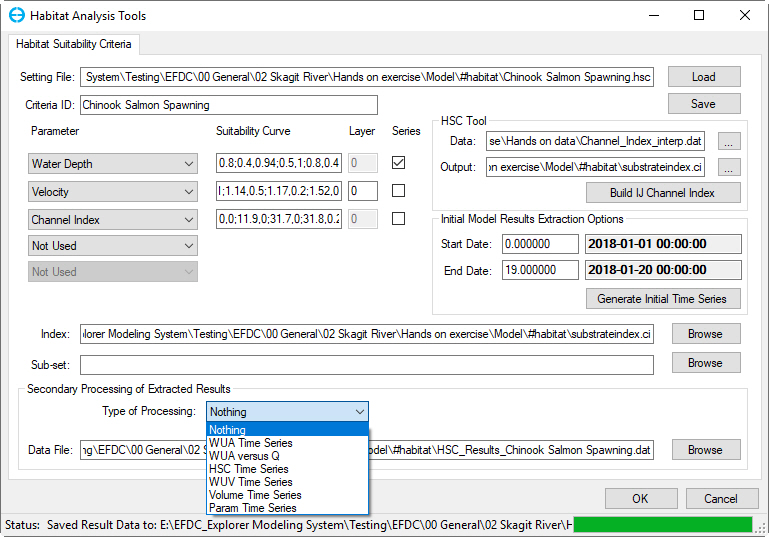
Once a time series has been generated, and the post-processing files have been extracted, a new frame is displayed, Secondary Processing of Extracted Results as shown in Figure 3.
Figure 3 Suitability Criteria: Secondary processing.
The drop-down menu for Type of Processing has the following options:
- WUA Time Series: This is a time series of the weighted usable area
- WUA vs Q: For this option the user must create a time series versus flow curve. This curve should match the initial boundary conditions that are being applied to the model. The user should enter the time versus flow (T vs Q) as x, y points in the table. EE will extract the WUA for the flow at this time and plot WUA vs flow.
- HSC Time Series: This is a number from 0 to 1 that is weighted over the entire domain.
- WUV Time Series: time series of weighted usable volume
- Volume Time Series: time series of volume
- Parameter Time Series: Depending on which option with a check box has been selected (only one at a time may be selected), EE will extract the time series for that parameter
After selecting one of these options EE will display a button to the right of the menu. Selecting this button will display the time series such as that for the WUA time series shown in Figure 4. If the user has extracted the results previously in this session, and then wants to view another secondary processing type, EE will prompt whether to use the data in memory, or whether to extract the data again.
Figure 4 Weighted Usable Area time series.
View Habitat Suitability Index in 2DH View
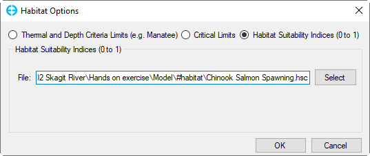
Once a time series has been generated, user can go to 2DH View window to view the habitat suitability index of each cell change by the time. From 2DH View window, users press keystroke Ctrl + H to open Habitat Options form as shown in Figure 5. From this form, select Habitat Suitability Indices option then click on Select button to browse to *.HSC file.
Figure 5 Habitat Options form.
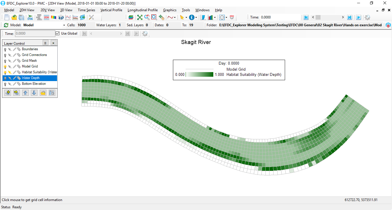
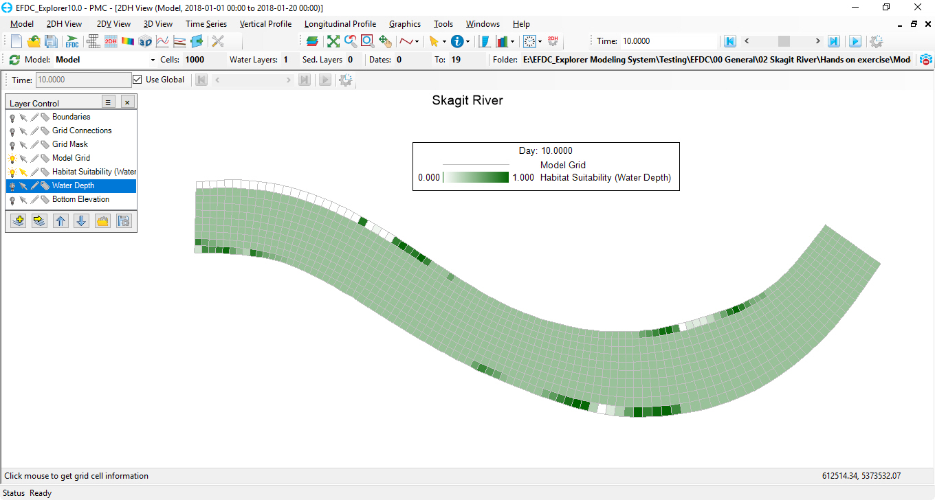
Habitat Suitability index of the interested species will be displayed at each time step as shown in Figure 6 and Figure 7 below.
Figure 6 HSC results at time step 0 in 2DH View.
Figure 7 HSC results at time step 10 in 2DH View.
