...
EE has the ability to add multiple winds, atmospheric, and ice stations. Stations may be defined and edited with the Edit button as shown in Figure 12. The user may also set a number of wind drag options from the Drag Options dropdown box, including Original, Original Relative U/V, Hersbach 2011 (ECMW), and COARE3.6 Simplified. The Original Relative U/V option computes wind drag using the original EFDC wind drag approach but takes into account the surface water velocities. The other two show the technical reference for their respective approaches.
| Anchor | ||||
|---|---|---|---|---|
|
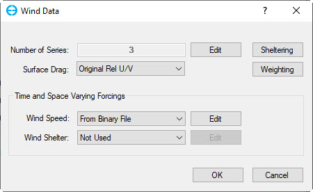
Figure 12. Hydrodynamics Option: Wind Data.
The user may set the coordinates of the wind series with the Show Params button in the Wind BC Time Series Editing as shown in Figure 23. EE will use the X and Y coordinates in the value column for display purposes. If the user has not entered the X and Y values, then EE will automatically calculate X and Y coordinates based on the lat/long values provided. However, if both are entered, it should be noted that EE will use the X and Y coordinates.
| Anchor | ||||
|---|---|---|---|---|
|
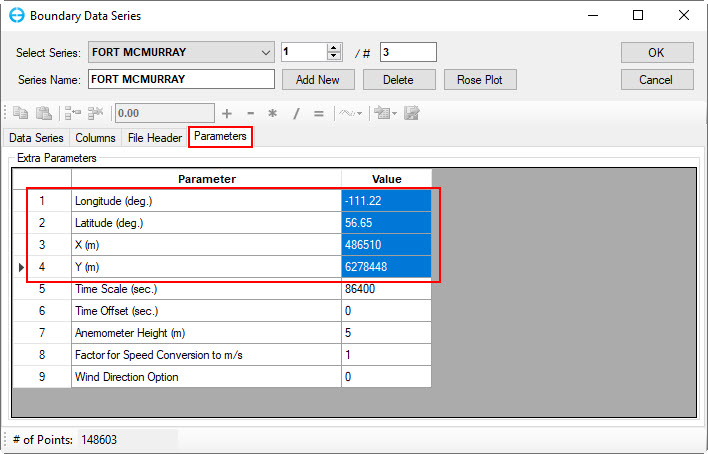
Figure 23. Wind Data Series: Station Coordinate Setting.
...
EE provides a flexible station weighting methodology for map files when handling multiple atmospheric series, wind series, and ice series. Each of these time series has a corresponding map file when there are multiple series. Calculation EE handles the calculation of the station weighting is handled by EE , and the input files for EFDC use the format described below. The series weighting provides weighting gives users with a simple tool for managing the data and stations for wind, ice, and atmospheric data. This approach allows EE to display the stations in a grid format with a quality index that indicates how the user rates each time series and time block within that series.
An example of a model domain with three wind stations is shown in Figure 34. This example has three stations WSER_1, WSER_2, and WSER_3. These have a total of different six-time series for wind, as shown in Figure 45.
| Anchor | ||||
|---|---|---|---|---|
|
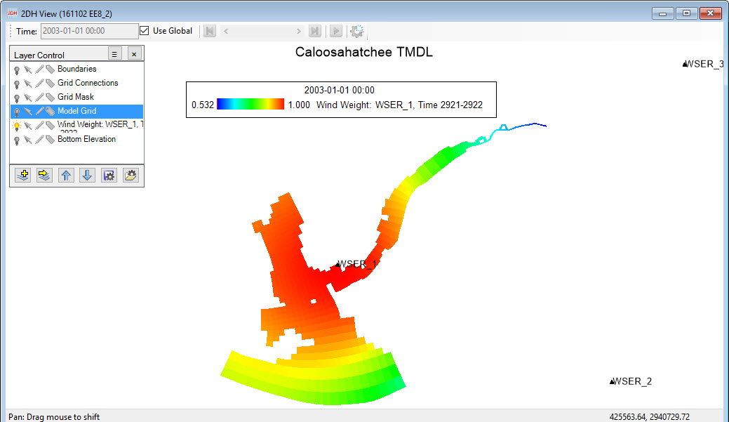
Figure 34. Wind weighting in 2DH View.
| Anchor | ||||
|---|---|---|---|---|
|
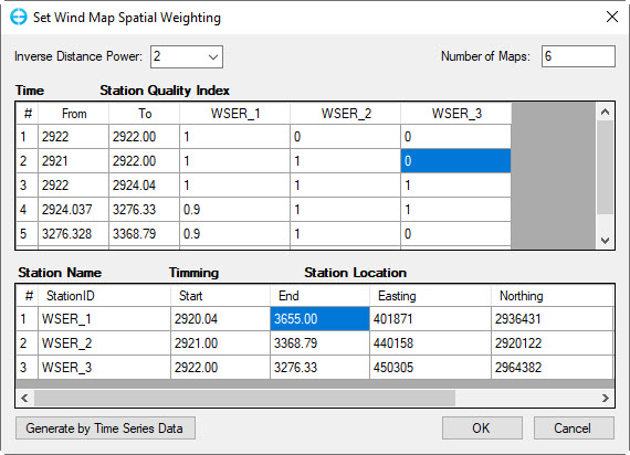
Figure 45. Wind Map: Default quality indexes for wind stations and time series.
In Figure 4, the default quality indexes have been set by EE after selecting the Generate by Time Series Data button. EE automatically generates the quality index with the maximum value of one for the defaults, which is 1. The user now needs to provide each time series with a quality index from 0 to 1. This weighting is based on users' judgment of the quality of this data series based on various factors. If the user knows of no problems with the series, then they would give it a rating of 1. However, often various factors will influence the quality of a time series and cause the user to downgrade the series, such as the distance from the model domain , or an intervening geographical feature. In this case, a lower value for the quality index will be selected. If another time series is available for that period with a higher weighting, it will have a greater impact on the model.
Each time series can be separated into many parts to set different quality/influence levels if necessary. EE will use the values provided in the Wind Map Spatial Rating table to generate the WNDMAP.INP file, an example of which is provided in the appendix. This file contains the calendar interval (Julian day) for which the following map is valid, and then the on each row is I, J, and weighting for each time series. This makes the format similar to EFDC GVC WNDMAP.INP file, however, it should be noted that GVC has certain specific requirements for these header files (six comment lines only). In a similar way, atmospheric series (ASER.INP), and ice series (ISER.INP) have map files which are ATMMAP.INP and ICEMAP.INP, respectively.
...
A wind rose plotting function is now available within the data series editing form for winds. Selecting the Wind Rose button as shown in Figure 5 6 prompts the user to input the start and end time for the rose data set to be displayed. After entering these data, the wind rose is displayed as shown in Figure 7.
| Anchor | ||||
|---|---|---|---|---|
|
...
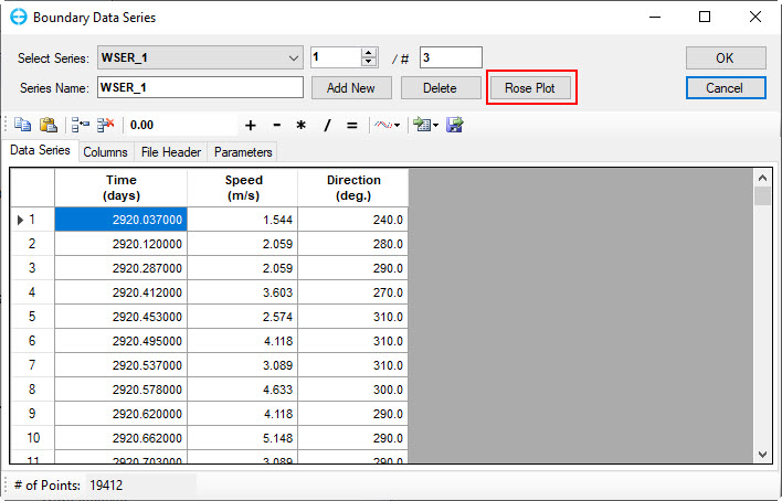
Figure 56. Boundary Conditions: Rose Plots for Winds.
| Anchor | ||||
|---|---|---|---|---|
|
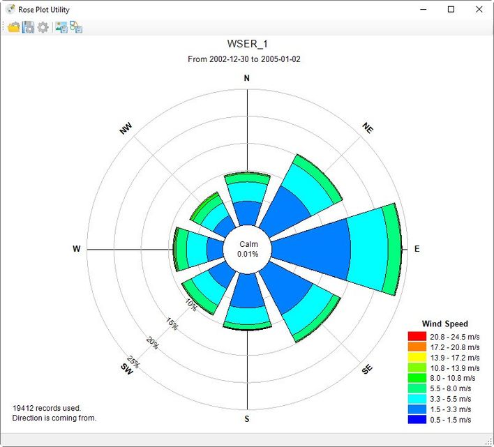
Figure 67. Example of a Wind Rose Plot.
A number of export functions are provided, including metafile and bitmap. The user can also customize the rose format by RMC on the rose and click on Setting or click on the setting button in the toolbar 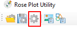 . The Rose Settings window is shown in Figure 78.
| Anchor | ||||
|---|---|---|---|---|
|
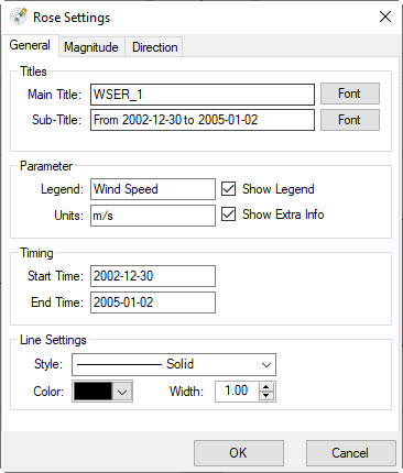
Figure 78. Rose Plot Settings.