Activate the Sediment Module
The Graphical User Interface (GUI) for the Sediment module in EE can be activated from the EFDC+ Modules, as shown in Figure 1.
| Anchor | ||||
|---|---|---|---|---|
|
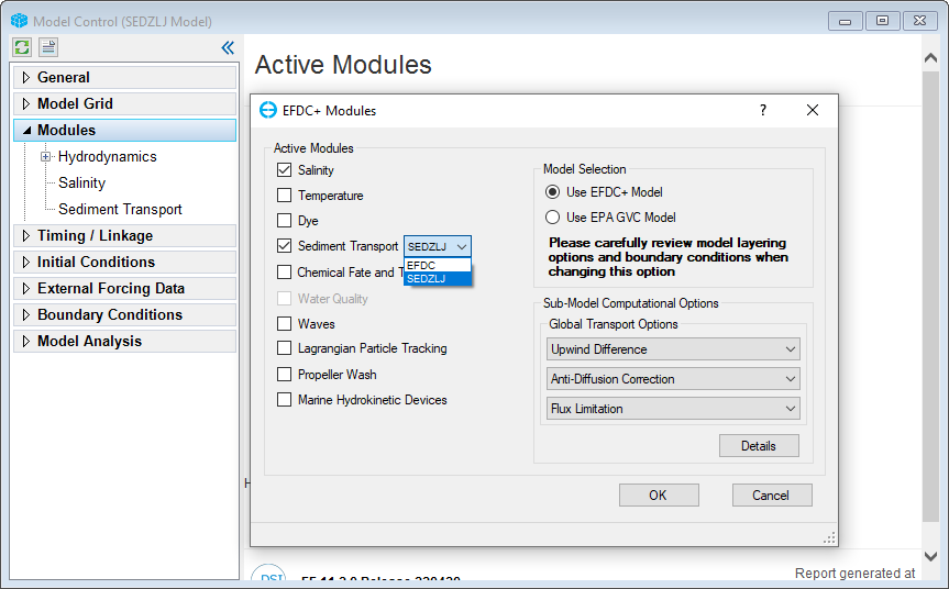
Figure 1 EFDC Modules Form - Sediment Transport Option.
...
Visualize Sediment
2DHView
The sediment can be visualized and animated in 2DH View. These can be added to the 2DH View by clicking the Add button in the 2DH View’s Layer Control then select Primary Group: Sediment Bed as shown in Figure 2. For the original sediment EFDC, the parameters include Bed Top Layer, Bed Thickness, Bed Density, Bed Porosity, Bed Mass, Bed Mass Fraction, Bed d50, Bed Delta and Bed Topography.
...
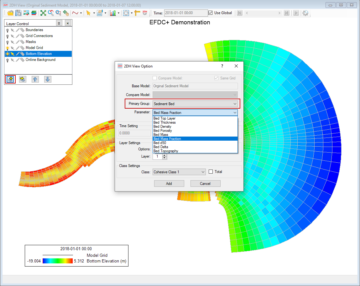
Figure 2. Original Sediment Bed Layer in 2DH View.
In the Layer Settings, it is able to select the display for all layers, top layer or for specific layer or depth as shown in Figure 3.
...
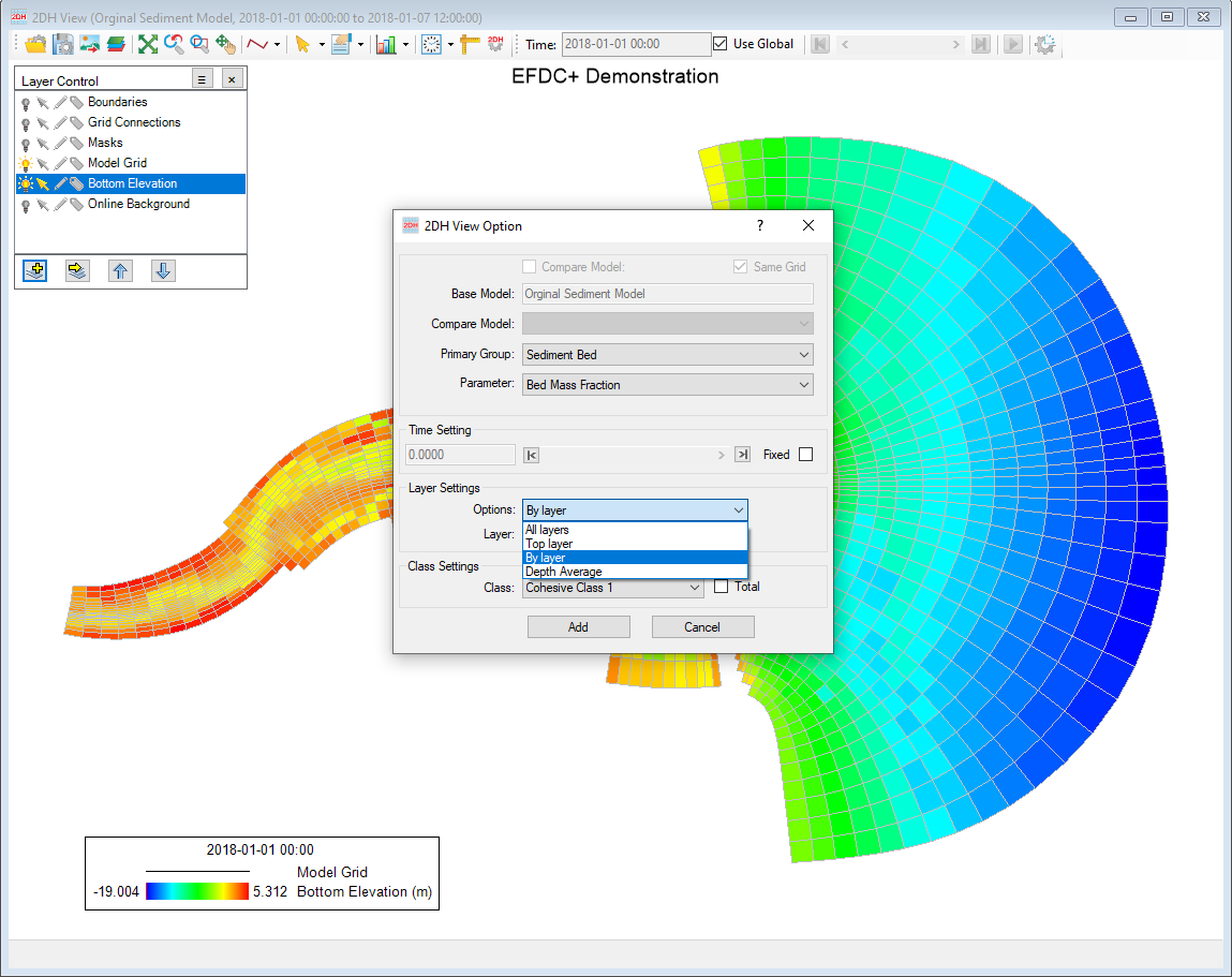
Figure 3. Layer Settings for Sediment Bed Layer in 2DH.
When the model contains multiple classes, EEMS supports to present the parameter for each class in 2DH View by selecting the class settings as shown in Figure 4.
...

Figure 4. Class Settings for Sediment Bed Layer in 2DH.
In term of sediment SEDZLJ model, the model output of SEDZLJ Sediment Bed are available to present in 2DH View. The parameters include SEDZLJ Core ID, SEDZLJ Skin Friction, SEDZLJ D50, SEDZLJ Erosion Rate, Net Deposition, SEDZLJ Bedload Chemical Fate and Transport, SEDZLJ Bedload Flux, SEDZLJ Bedload Vector and SEDZLJ Bedload Mass.
...
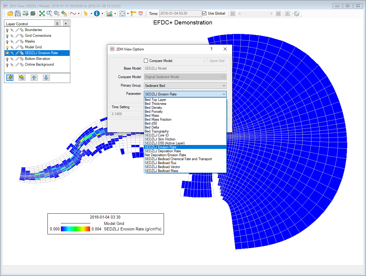
Figure 5. Sediment SEDZLJ Layer in 2DH View.
Time Series
The graphic of sediment bed time series can be visualized by click the Time Series button or the icon ![]() of the main toolbar. The Extract Time Series Data tab appears as shown in Figure 6. It is possible to plot the time series for a single cell or multiple cells. Firstly, defying the cells to plots is in the box under Selected Cells. When the L index is entered the corresponding I and J indices are filled automatically. The parameter should be defined in the box, Primary Group: Sediment Bed and then the drop-down list of parameters is available. Add and remove the parameter can be adjust by the left and right arrow button. The user may define the start and stop day for the time series in Time Series Start/Stop frame (note that the start and stop days should be within the model's start and end date). Clicking OK plots the selected graphs
of the main toolbar. The Extract Time Series Data tab appears as shown in Figure 6. It is possible to plot the time series for a single cell or multiple cells. Firstly, defying the cells to plots is in the box under Selected Cells. When the L index is entered the corresponding I and J indices are filled automatically. The parameter should be defined in the box, Primary Group: Sediment Bed and then the drop-down list of parameters is available. Add and remove the parameter can be adjust by the left and right arrow button. The user may define the start and stop day for the time series in Time Series Start/Stop frame (note that the start and stop days should be within the model's start and end date). Clicking OK plots the selected graphs
...
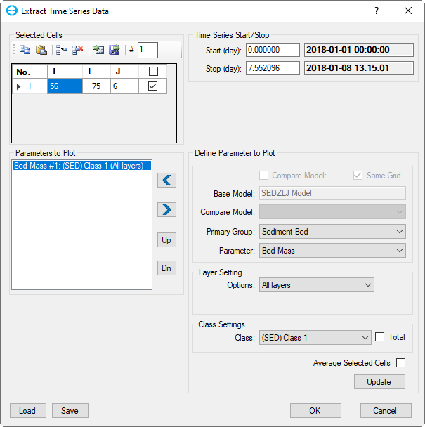
Figure 6. Extract Time Series Data.
...
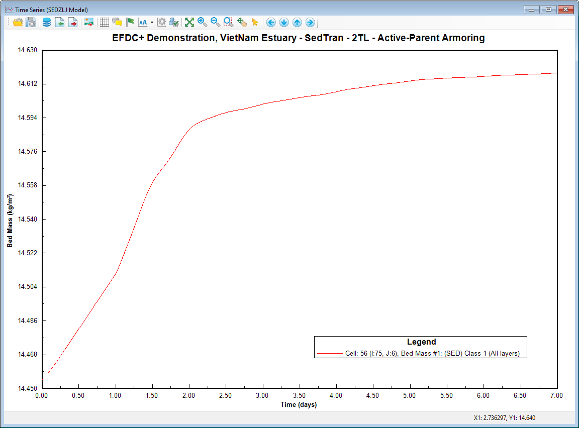
Figure 7. Sediment Bed Thickness Time Series
Longitudinal Profiles
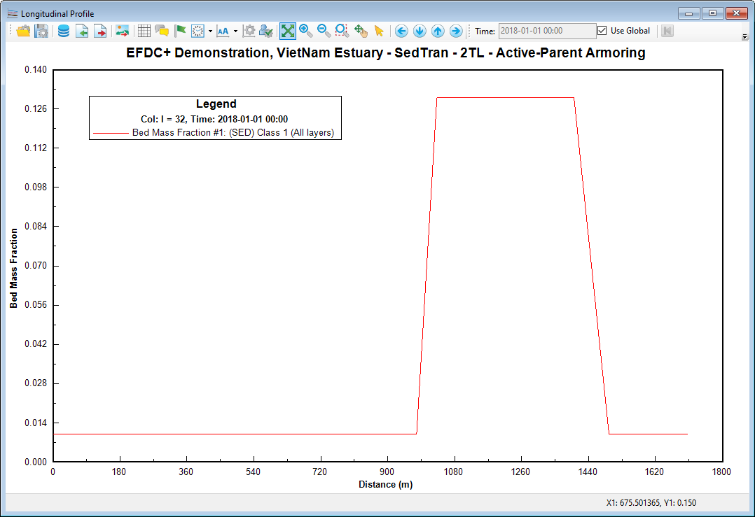
The graphic of wave longitudinal profiles can be visualized by click the Longitudinal Profile button or the icon ![]() of the main toolbar. Figure 8 show the Data Extraction for Longitudinal Profile form. This form is similar to the Data Extraction for 2DV View form. Firstly, it is necessary to define the profile using drape file or I, J indices and then defines the parameter to the plot. The parameter should be defined in the box, Primary Group: Sediment Bed . Add and remove the parameter can be adjust by the left and right arrow. Once everything is ready, click OK to generate the plot. Figure 9 shows a longitudinal profile for wave height and bottom elevation along the profile I=81
of the main toolbar. Figure 8 show the Data Extraction for Longitudinal Profile form. This form is similar to the Data Extraction for 2DV View form. Firstly, it is necessary to define the profile using drape file or I, J indices and then defines the parameter to the plot. The parameter should be defined in the box, Primary Group: Sediment Bed . Add and remove the parameter can be adjust by the left and right arrow. Once everything is ready, click OK to generate the plot. Figure 9 shows a longitudinal profile for wave height and bottom elevation along the profile I=81
...
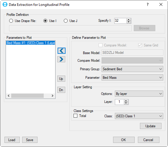
Figure 8. Data Extraction for Longitudinal Profile
...
...