The EFDC_DSI/EFDC_Explorer system has the ability to easily compute a residence time or "Age of Water". This function uses the dye sub-model for simulation. The theory behind the function and a step-by-by approach for how to use this feature is provide below.
Age of Water Approach
The age of water approach uses the DYE constituent, referred to as "age" in days. The transport equation for the AGE constituent having an "age" (equivalent to a "mass") per unit volume C, is:
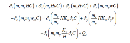
Where:
C represents the AGE;
Qc represents the source term for age, at all active cells for each time step
Qc = delta T, in days
So, at the end of the advection and diffusion step the source term is added for the time step resulting in:
Ct+1 = Ct + delta T
The result is C (i.e. AGE) in days output in the water column for each snapshot.
Step by Step Instructions
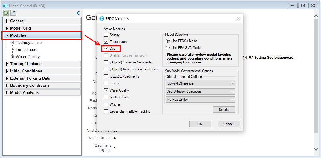
Step 1: Active DYE module in Modules tab
From Model Control form, RMC on Modules tab, select Active DYE
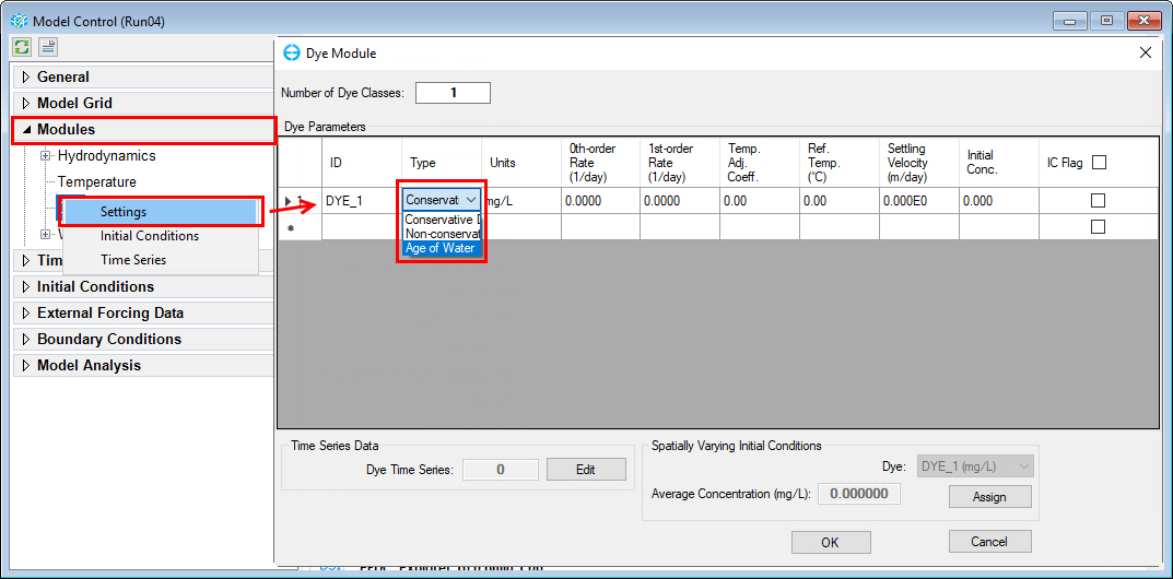
Step 2: Assign the Age of Water Flag to the Dye Decay Rate
From Model control form, RMC on DYE under Modules tab, select setting to open DYE module form. From DYE module form, click on dropdown menu under type column and select Age of Water to effectively treat the dye constituent as an age counter. Every timestep the dye constituent is transported in a method similar to all other water column constituents. At the end of the dye transport the water is "aged" by adding the delta-T in days, to the dye constituent. The result is the dye constituent represents the age of water in days.
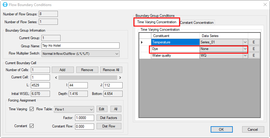
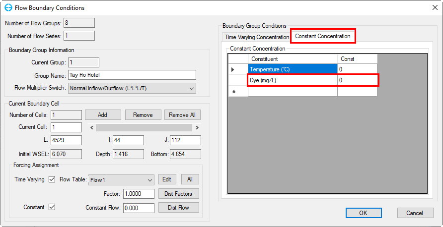
Step 3: Zero Dye Boundary Conditions
The standard approach is to assume that all incoming water to the model domain has an age of zero days, i.e. "new" water. To do this the user should set all boundary condition dye concentrations and/or series to 0. The following is an example of the flow boundary type. The same approach would be used for pressure or withdrawal/return.
Step 4: Save the Project
Step 5: Run the Project
Step 6: Post Processing:
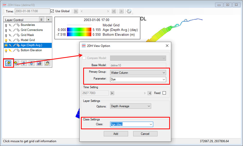
Go to 2DH View window and select Add New Layer button will bring up 2DH View Option form. From 2DH View Option form, select Water Column in Primary Group frame, Dye for Parameter, in Class Settings frame, select Age (day) class to add Age of water layer in 2DH View . The user can generate animations, longitudinal profiles, vertical profiles, etc. as with any water column constituent.
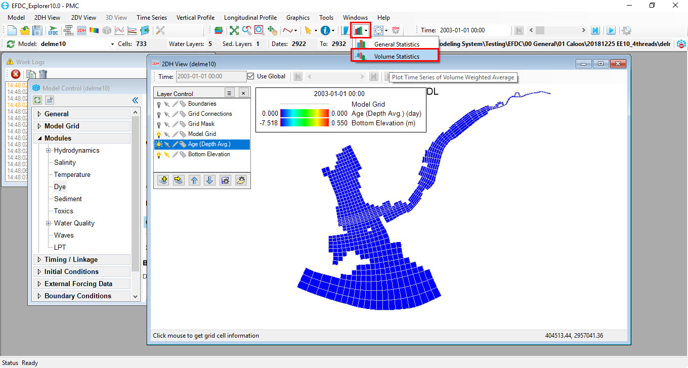
Step 7: Post Processing: Generate Time Series of Mass Weighted Age
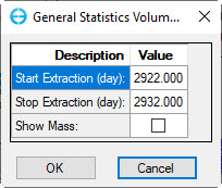
Once the user is viewing the Age of Water option (see Step 6) they may want to generate a time series of the average age of water for the whole model or some selected area. This can be done by select Age layer under Layer Control form then selecting the Volume Statistics tool from the toolbar (see below).
EE will pop-up General Statistic Volume Start/Stop form which allows user define the extract time period. The initial default is the entire model simulation period. However, the user can select only the period of interest. Moreover, user can select show mass loading or not by select checking or unchecking on Show Mass checkbox.
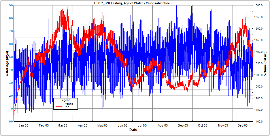
Once the time series extractions have been completed EE will display a plot of the results. The following shows the results of the time series extraction of "Age of Water" for the entire model domain. The Age (red line) is plotted against the left axis, the volume of water is plotted against the right axis.
The user can then extract the data as an ASCII file or filter the data (press F2 to see options). The ASCII extraction tool is highlighted below:

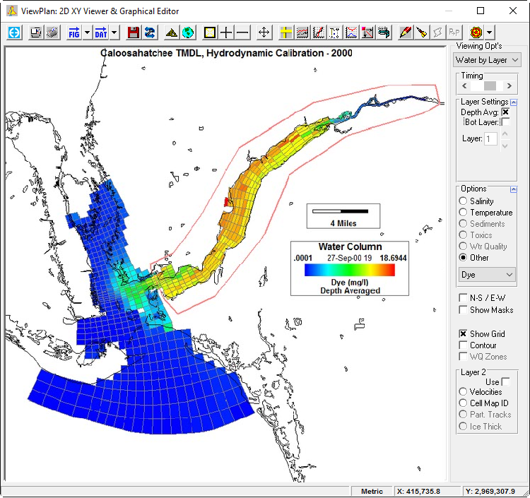
The following screen capture shows the Caloosahatchee-San Pablo Bay model domain with a cell selection polygon for the Caloosahatchee Estuary overlaid on the model domain.
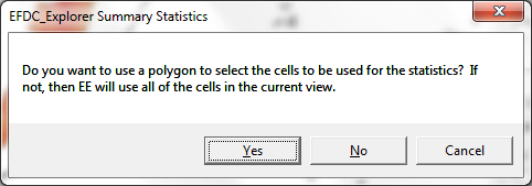
If the user selects the option to use a cell selection polygon, they will be requested to enter one.
The following plot shows the "Age of Water" extraction from both the entire model domain as well as using the cell selection polygon to extract the age from only the Caloosahatchee Estuary.

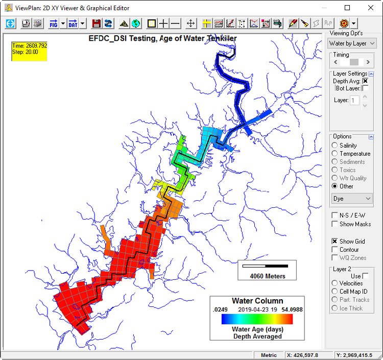
Lake Example - Ten Killer Lake, Oklahoma, USA
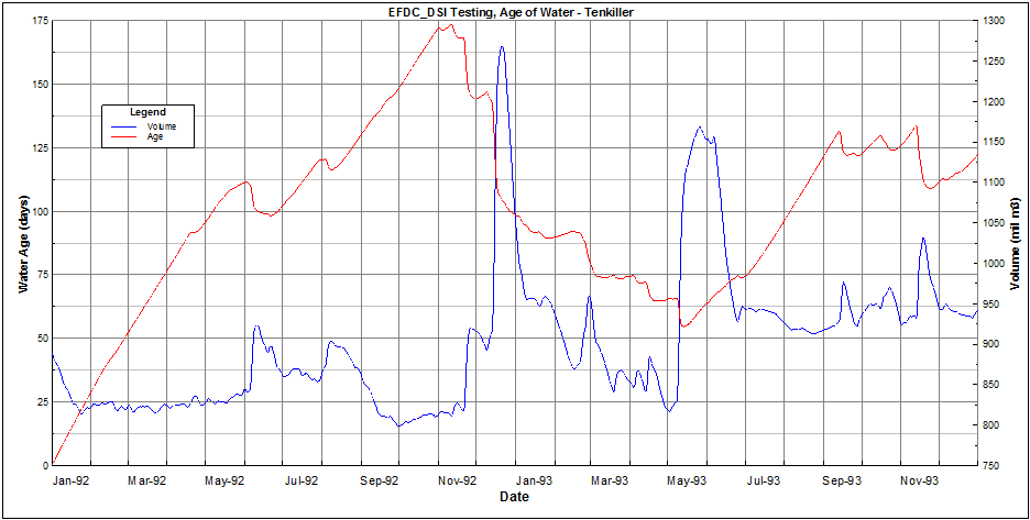
The Age of Water will be dependent on the inflows and outflows and will vary from year to year. A two year simulation was performed and then the mass weighted Age of Water for the entire domain was extracted. The results are shown in the following plot.
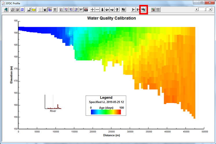
A vertical slice extraction of the Age of Water along the centerline line shown on the Tenkiller grid map above is shown below. The user may also animate this image using the animate tool which shows the clear effects of density stratification and density currents.