In the 2DH View window, EE10 has the option of setting the layer properties displayed on the legend. This can be achieved by RMC on the selected legend in Layer Control frame.
Figure 1 shows Properties option from RMC on the Bottom Elevation layer as an example. When Properties is selected the Layer Properties form is displayed as shown in the Figure 2. The options on this form vary depending on the specific layer being selected. An example of two forms are shown in Figure 2 and Figure 3 for bottom elevation and Model Grid layers respectively. The various options in these forms are described in more detail below. A wide variety of options are available for displaying and exporting data when the user RMC's on the Bottom Elevation in the Layer Control, as shown in Figure 1. These options are described below.
| Anchor | ||||
|---|---|---|---|---|
|
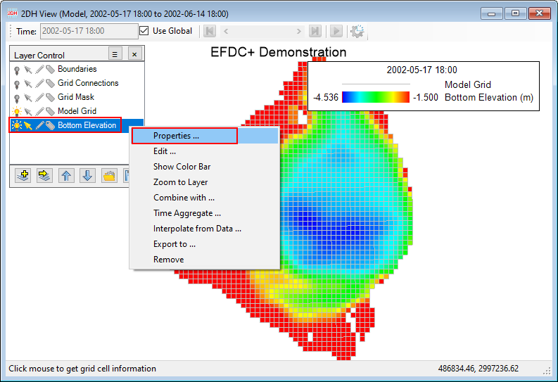
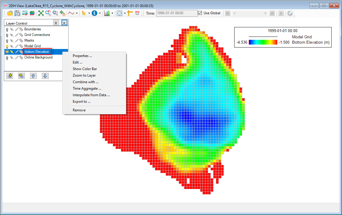
Figure 1. Layer properties option of bottom elevationBottom elevation: RMC options.Anchor
...
Properties
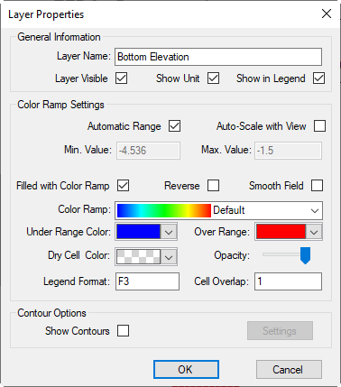
When Properties is selected the Layer Properties form is displayed as shown in the Figure 2.
3Anchor Figure
32 Figure 2
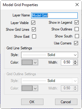
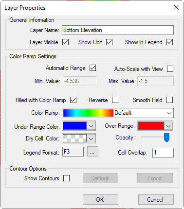
Figure 32. Layer Properties for Model Grid layerform.
The Layer Properties forms have form has the following options:
General Information
...
Layer Visible: Checking this box allows the layer to be seen in the 2DH View, and s has the same effect as toggling the layer by turning on/off the light bulb.
...
Color Ramp: When the Filled with Color Ramp box is checked, the user can select different color ramp options from the drop-down list. The options available are shown below. Options such as Viridis and Plasma are provided to more accurately represent certain data types. These saturation/lightness change linearly and are colorblind-friendly.
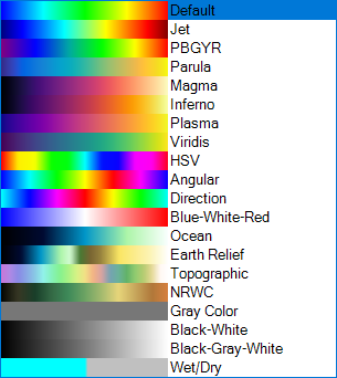

Figure 43. Color Ramp options.
Under Range Color: Set a color for values that are less than the Min. Value
...
Legend Format: This is used to set the significant figures for the minimum, and maximum values displayed on the legend. As default, EE sets F3 for this field. However, the user can change this by double-clicking on the box and the Number Format form will be displayed as shown in Figure 54. The user can change Decimal Digits by entering a number or using the Up and Down arrows (e.g 0 - integer number, 1 - one decimal digit, 2 - two decimal digits, etc).
...
Show Contours: Check on this box to show the value contours of the layer. If it is checked, the Settings and Export options will be enabled.
Settings: To set contour settings
...
Export: To export contour lines to a file
When displaying the bottom elevation from the Layer Properties settings a legend is displayed. The different elements of 2DH legend are shown in Figure 5.
| Anchor | ||||
|---|---|---|---|---|
|
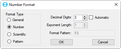
Figure 4. Number Format form.
| Anchor | ||||
|---|---|---|---|---|
|
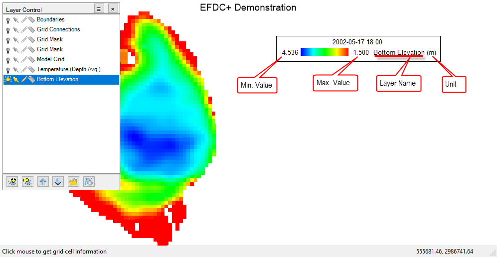
Figure 5. Number Format form.. Display of Bottom Elevation on the Legend.
Edit
Selecting this option, the user can change the current layer to another layer by selecting from the drop-down list in the Primary Group and Parameter.
Show Color Bar
This option will show a color bar for the bottom elevation; as default, a vertical color bar is added to the 2DH View as shown in Figure 6.
The user can edit the color bar by RMC as shown in Figure 7.
Settings: From the Color Bar Settings form, the user can change the title and font size of the title, change decimal digits and font size of value labels, change the number of ticks on the bar as shown in Figure 8.
Vertical Direction: Show the Color Bar in the vertical direction.
Horizontal Direction: Show the Color Bar in the horizontal direction.
Auto-fit Title: In case the title's font size is too large, and it is covered by the color bar frame, using this option will adjust the frame to fit the title length.
Hide: Use this option to hide the color bar.
| Anchor | ||||
|---|---|---|---|---|
|

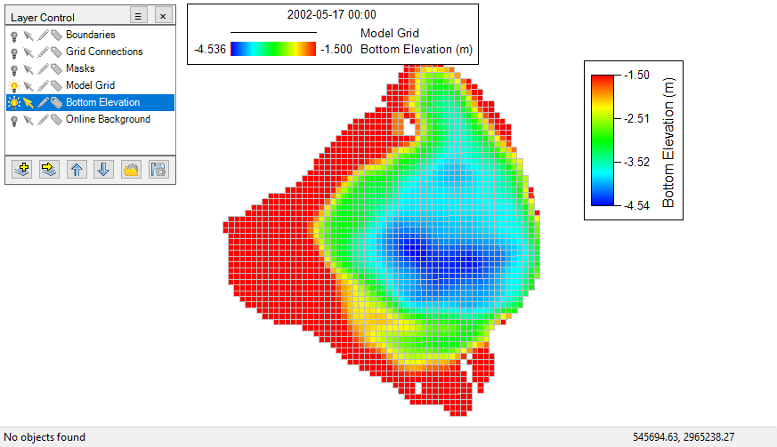
Figure 6. Display of Bottom Elevation on the Legend. Color bar of Bottom Elevation.
Anchor Figure 7 Figure 7
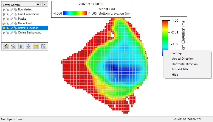
Figure 7. RMC options of the Color bar.
Anchor Figure 8 Figure 8
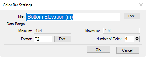
Figure 8. Color bar: settings.
Zoom to Layer
Zoom to view the full extent of the Bottom Elevationlayer.
Combine with
When this option is selected, the Composite Layer form will appear, as shown in Figure 9. The options include:
Base Layer: This is the selected layer that was RMC'd on, and it cannot be changed in this form.
Secondary Layer: This layer can be selected from the dropdown list when is it available in the Layer Control.
Resultant Layer Equals: This is an equation that can be selected from the dropdown list. Note the user should define a proper equation for the two layers.
Resultant Layer Name: This is the name of the resultant layer, and may be edited. By default, the name is taken from the Resultant Layer Equals above.
Resultant Units: This is a unit for the resultant layer. A proper unit can be entered in this field.
Anchor Figure 9 Figure 9
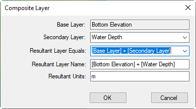
Figure 9. "Combine with" form.
Time Aggregate
When this option is selected, the Time Aggregation form will appear, as shown in Figure 10. The options available include:
Base Layer: This is the selected layer that was RMC'd on.
Options: Various options may be selected from the dropdown list such as None, Average, Cumulative, Minimum, Maximum, Time Integration.
Begin: This is the beginning time, from the Date Start of the Model Timing as default.
End: This is the ending time, from the Date End of the Model Timing as default. Note that the user can enter a new Begin and End time. However, it needs to be between the Date Start and Date End of the Model Timing.
Secondary Layer: This layer can be selected from the dropdown list when is it available in the Layer Control.
Layer Name: This layer is created based on selecting the above option. The user can define a new name for this layer.
Click the OK button, a new layer is created and added to the Layer Control.
Anchor Figure 10 Figure 10
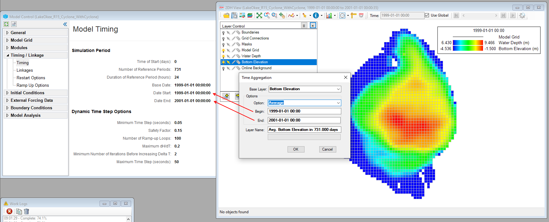
Figure 10. Time Aggregate.
Interpolate from Data
This option allows for interpolating the selected layer from a data file; the data file is added to the Layer Control (e.g., contours).
From the Data Interpolation form (Figure 11), select the layer to interpolate from the dropdown list for Interpolate for, check the box to select the data file in the Data sets for interpolation, then click the OK button. In this case, suppose that the initial bottom elevation was set to 0. After clicking the OK button, the bottom elevation of the model will be updated (Figure 12). To retain the updated bottom elevation for the model, save the model to a new one or export the bottom elevation layer to an external file for later use.
Anchor Figure 11 Figure 11
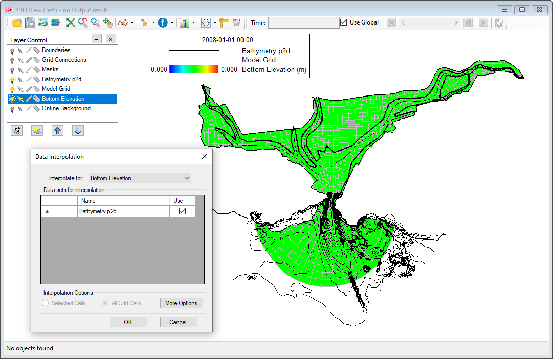
Figure 11. Interpolate from Data (1).
Anchor Figure 12 Figure 12
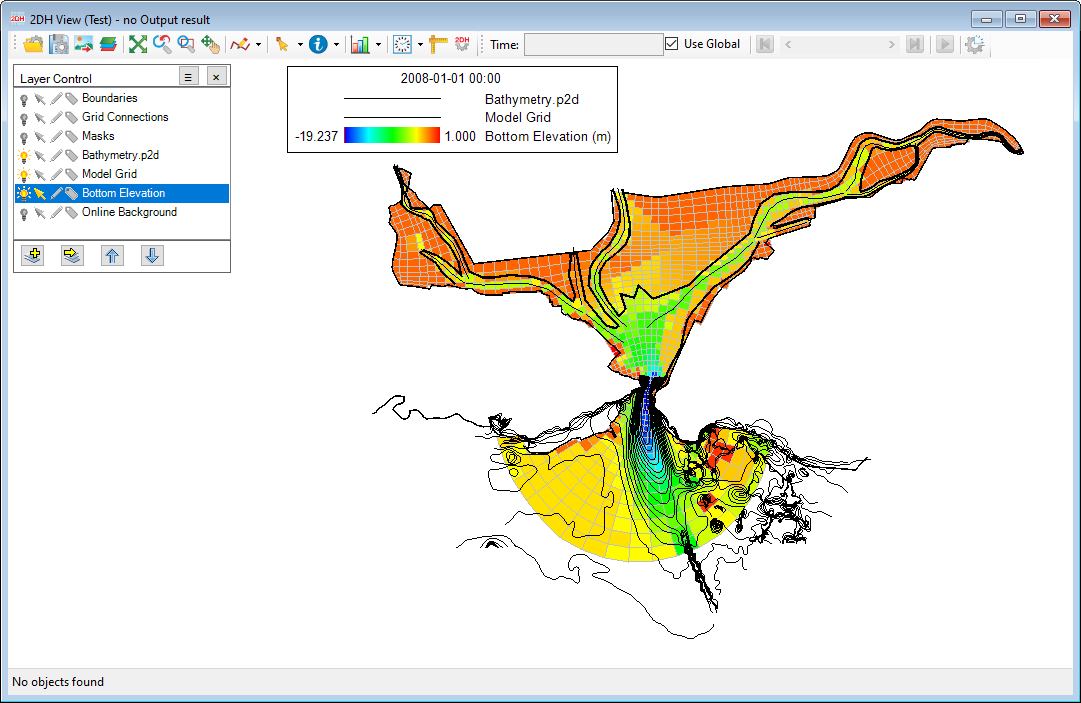
Figure 12. Interpolate from Data (2).
Export to
This option will export the bottom elevation of the model to an external file, and the file extension can be varied by selecting from the drop-down list for the Save as type. The file contains the cell's centroid coordinate (X, Y) and bottom elevation (Z).
Remove
Remove the Model Grid layer from the Layer Control frame.