Table of Contents
1 Introduction
2 Create a New Grid
3 Assigning the Initial Conditions
3.1 Assigning the Initial Bottom Conditions
3.2 Assigning the Depth/Water Surface Elevations
3.3 Assigning the Bottom Roughness
4 Assigning the Boundary Conditions
4.1 Preparing the Flow Boundary
4.2 Preparing the Tidal Level Boundary
4.3 Assigning Time Series to the Boundary Location Cells
4.3.1 Assigning the Flow Boundary
4.3.2 Assigning Tides Boundary
5 Hydrodynamics Settings
6 Setting Vertical Layers
7 Model Timing
8 Running EFDC+
9 Visualizing the EFDC Solution
| Anchor | ||||
|---|---|---|---|---|
|
This tutorial document will guide you how to setup a coastal hydrodynamic model by using the EFDC_Explorer (EE). It will cover preparation of the necessary input files for the EFDC model and visualization of the output by using the EFDC_Explorer (EE) Software.
The data used for this tutorial are from Tra Khuc Estuary in Vietnam. All files for this tutorial are found in Data folder downloadable from the EEMS website.
Before going to each session, let us first introduce the EE main form in order to better understand our explanation hereafter. Figure 1 is the main form of EFDC_Explorer or EE User Interface. The functions of individual icons are described in Knowledge Base.
| Anchor | ||||
|---|---|---|---|---|
|
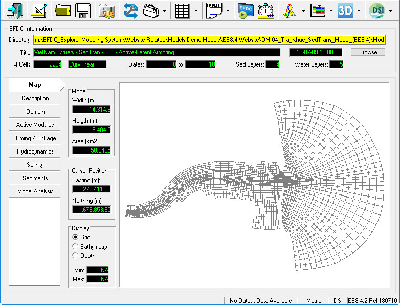
Figure 1 EFDC Explorer main form.
| Anchor | ||||
|---|---|---|---|---|
|
This section will guide you in how to create a new simple gird with EFDC_Explorer. For a complicated grid the user is recommended to use specialized grid generation software such as CVLGrid or Delft3D-RGFGRID.
Tra Khuc Estuary in Quang Ngai province, Vietnam is chosen as the example of building a 3D coastal model in EE.
The gird generation process includes following steps:
- Open EE
- Click Generate New Model icon as
 on the main menu of EE interface. Then Generate EFDC Model frame appears shown in Figure 2
 - Select CVLGrid in the Grid Type. The user should click the Browse button to select grid file name as Trakhuc.cvl in Grid folder sas as shown in Figure 2. In the other hand, EE also supports the user to import various format of grid file with the option Import Grid.
- Click Generate button in Figure 2 to to finish. A dialog will pop up to show the grid information (see see Figure 3).
| Anchor | ||||
|---|---|---|---|---|
|
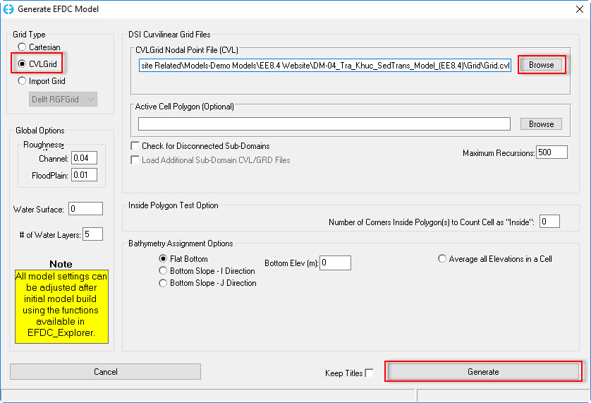
Figure 2 Generate EFDC Model form.
| Anchor | ||||
|---|---|---|---|---|
|
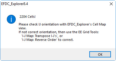
Figure 3 New created grid information.
5. Save the model by selecting this button  and create a new directory as shown in Figure 4.
| Anchor | ||||
|---|---|---|---|---|
|
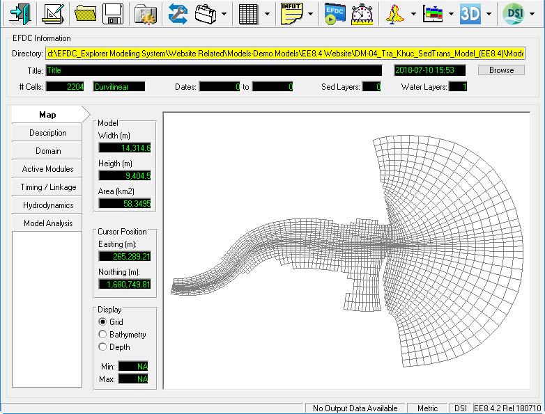
Figure 4 New model saved.
| Anchor | ||||
|---|---|---|---|---|
|
This section will guide you in how to assign the initial conditions such as the bathymetry, water level and bottom roughness.
| Anchor | ||||
|---|---|---|---|---|
|
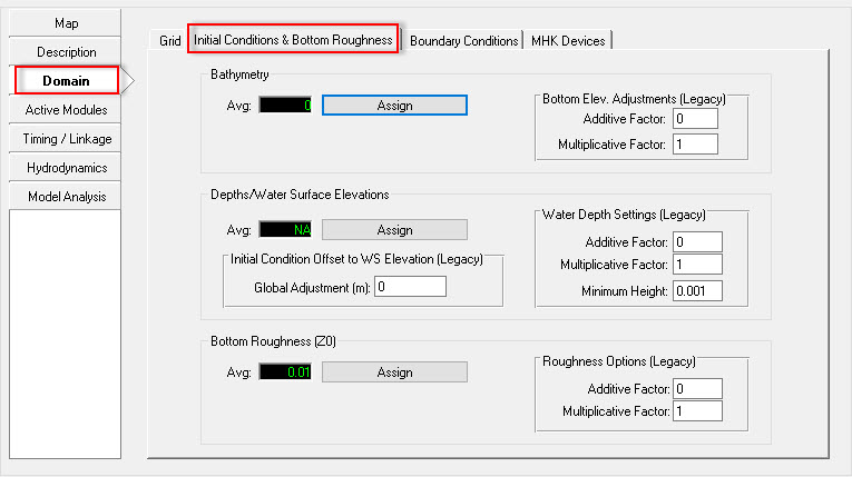
Figure 5 Assigning the initial conditions.
| Anchor | ||||
|---|---|---|---|---|
|
- Select the Domain/Initial Conditions & Bottom Roughness and click the Assign button (see Figure 5).
- A polyline file is used to define the area to assign the bathymetry data. To assign this browse in the Poly File form to "Domain.p2d".
- Next browse to the bathymetry data file in the Data File form. This bathymetry file is simply a general xyz format.
- There are a number of options for the for user to modify the assigned. In this case, we choose in the Bathymetry Assignment Options we select Interpolated Data and Both. This will take the nearest neighbor data points to interpolate for the cells where there is no data coverage.
- Click the Apply button to take the effect before hitting the Done button (see see Figure 6)
| Anchor | ||||
|---|---|---|---|---|
|
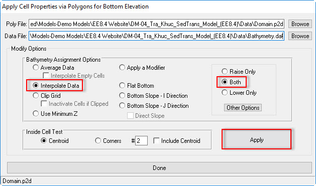
Figure 6 Assigning the bathymetry.
| Anchor | ||||
|---|---|---|---|---|
|
The next step is to assign the initial depth or water surface elevations. There are two options for setting the surface water elevation which are Use Constant and Use Point Measurements/Gridded Data.
- Click Assign button
- Browse in the Poly File form to "Domain.p2d"
- Next, browse to the water surface elevation data file "IC_WSEL.dat" in the Data File form.
- Checked on Use Point Measurements/Gridded Data
- The user click Apply button then click Done button to finish.
| Anchor | ||||
|---|---|---|---|---|
|
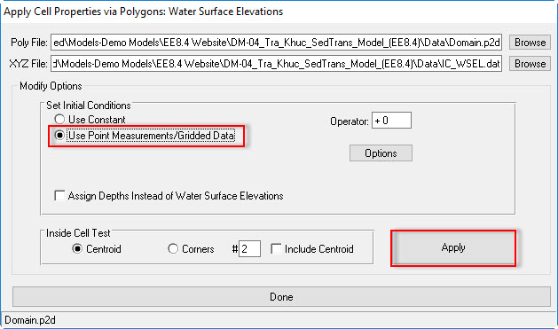
Figure 7 Assigning water surface elevation.
| Anchor | ||||
|---|---|---|---|---|
|
- Click the Assign button in the Bottom Roughness (Z0) box (Figure 5).
- Browse in the Poly File form to "Domain.p2d"
- Next, browse to the bottom roughness data file "IC Bot Roughness.dat" in Data folder in the Data File form.
- Checked on Use Point Measurements/Gridded Data
- Click the Apply button before hitting the Done button as shown in Figure 8.
| Anchor | ||||
|---|---|---|---|---|
|
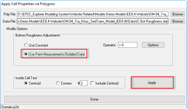
Figure 8 Assigning bottom roughness.
| Anchor | ||||
|---|---|---|---|---|
|
This section will guide you how to prepare for the boundary conditions and assign it to the model cell configuration. In this coastal case there are two flow boundaries; one is river discharge from the upstream and the other is tidal level. Thus, we should prepare two time series of inflow and tidal level boundaries for this particular case. In order to set a boundary time series the steps outlined below should be taken.
| Anchor | ||||
|---|---|---|---|---|
|
- Select the Domain/Boundary Conditions. (See Figure 9).
- Click to the E button
 which is next to Flow to edit the flow boundary. (Figure 9)
 - Enter the Number of Series into the box which in this case is 1.
- Give a Title for associated time series, in this case "River".
- Click Import Data button, browse to "BC_Flow.dat" file in Data folder
- Select EE DAT or WQ Data format then click OK button. (See Figure 10).
- Enter "-1" in Import Data form then click OK button. (See Figure 11).
Click to the Current button
 to view the current time series. If there are a number of layers then check Sum Layers to show total flow. (See Figure 1112). Close timeseries data plot
Click OK button in Data Series: Flow form to finish editing the boundary time series.
| Anchor | ||||
|---|---|---|---|---|
|
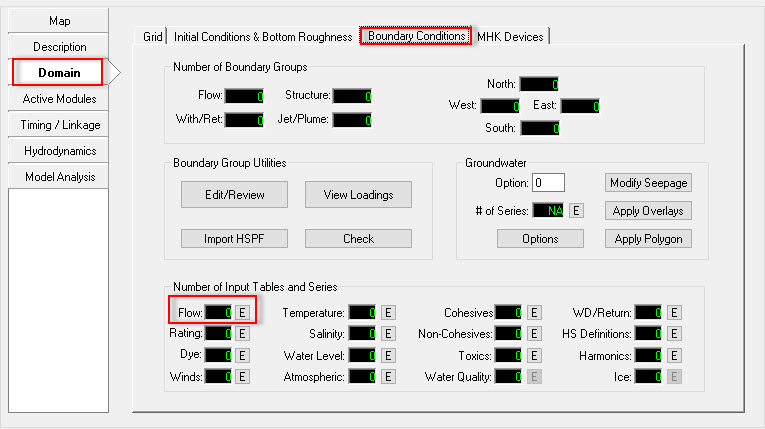
Figure 9 Assigning flow boundary conditions.
| Anchor | ||||
|---|---|---|---|---|
|
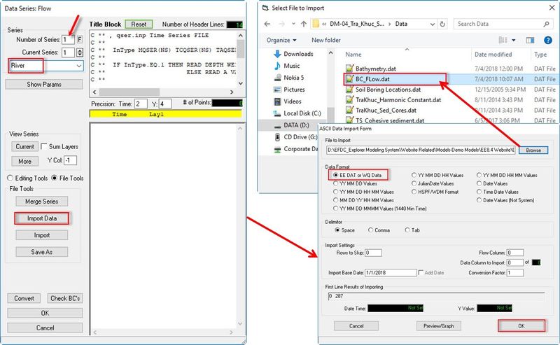
Figure 10 Editing the boundary time series (01).
Anchor Figure 11 Figure 11
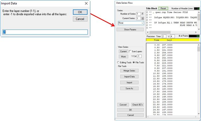
Figure 11 Editing the boundary time series (02).
| Anchor | ||||
|---|---|---|---|---|
|
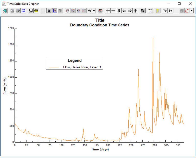
Figure 12 Flow time series plot.
| Anchor | ||||
|---|---|---|---|---|
|
- Click to the E button
 which is next to Water Level (See Figure 1213)
 - Enter the Number of Series, which is 1 for this case (see Figure 1314)
- Enter the Title of Series as "Tides"
- Open "BC_Water Level.dat" file in Data folder, the copy and paste into the Data Series: Water surface form.
- Click Current button in the form to see the timeseries plot (see Figure 1415). Close timeseries data plot.
- Click OK to finish.
Another option for setting the open boundary is the Harmonic Boundary Series (Harmonic Boundary Series)
| Anchor | ||||
|---|---|---|---|---|
|
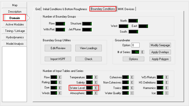
Figure 12 13 Assigning tidal boundary conditions.
| Anchor | ||||
|---|---|---|---|---|
|
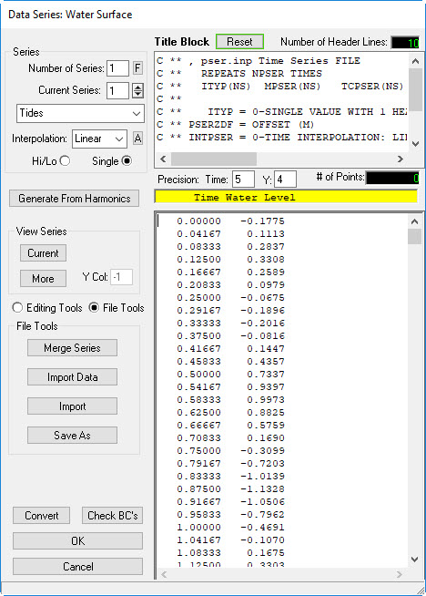
Figure 13 14 Preparing the tidal boundary series.
Anchor Figure 1415 Figure 1415
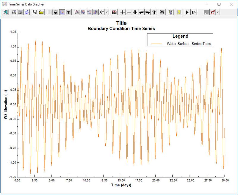
Figure 14 15 Tides time series plot.
| Anchor | ||||
|---|---|---|---|---|
|
When all required boundary time series are prepared the next step is to assign those boundary time series to the model cells. Figure 14 shows the location of inflow and tidal level for the TraKhuc case.
| Anchor | ||||
|---|---|---|---|---|
|
In order to assign the flow boundary, the following steps should be taken
- Click to the ViewPlan icon
 on the main form (See Figure 1516).
 - Choose Boundary C’s in the Viewing Opt’s
 .
. - Check Enable Edit and Show Grid (See Figure 1617).
- RMC on the inflow location cell/ choose New (See Figure 1718).
- Enter the boundary group ID: River (See Figure 1718).
- Select boundary types. It is dependent on your current boundary type to choose the suitable boundary type. In this case, we have a flow boundary so we choose number 1 (See Figure 1718).
- Select the associated times series for this inflow boundary, "Flow" (See Figure 1819).
- Click OK to complete.
- The boundary cells might have multiple cells to present the real river width. In order to assign the multiple cells, click Add by Polyline button in the form of Figure 1819, you need to browse to the "US_BC Line.p2d" in the Data folder as shown in in Figure 1920 then click Apply button.
- Click All button to assign river flows to all cells ( See Figure 2021)
- The inflow is now divided to the number of assigned cells. (See Figure 2122).
| Anchor | ||||
|---|---|---|---|---|
|
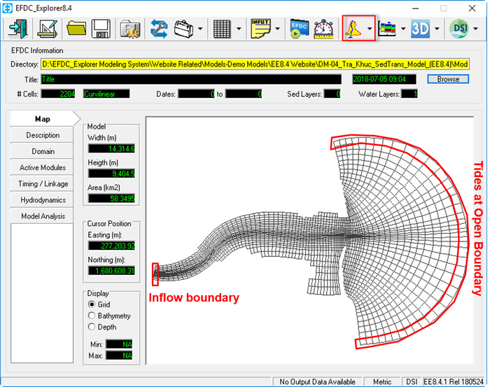
Figure 15 16 Locations of inflow and open tidal boundaries.
| Anchor | ||||
|---|---|---|---|---|
|
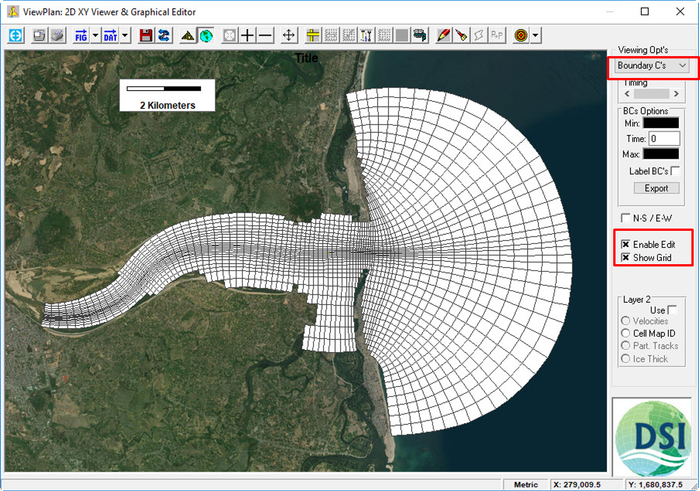
Figure 16 17 Assigning boundary condition cells.
| Anchor | ||||
|---|---|---|---|---|
|
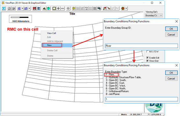
Figure 17 18 Create new boundary condition with RMC on the inflow cell.
| Anchor | ||||
|---|---|---|---|---|
|
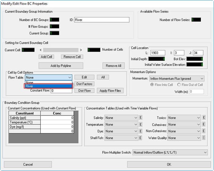
Figure 18 19 Assign the corresponding time series.
| Anchor | ||||
|---|---|---|---|---|
|
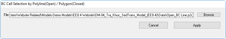
Figure 19 20 Assigning boundary cells by a polyline.
Anchor Figure 2021 Figure 2021
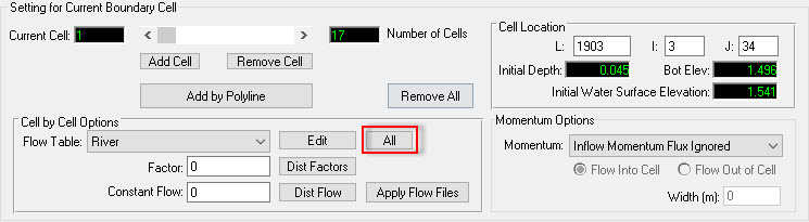
Figure 20 21 Assigning BC to all selected cells.
Anchor Figure 2122 Figure 2122
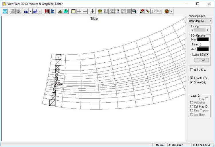
Figure 21 22 Upstream BC cells assigned.
| Anchor | ||||
|---|---|---|---|---|
|
In order to assign the tides boundary, the following steps should be taken:
- Click to the ViewPlan icon
 on the main form (See Figure 1516).
 - Choose Boundary C’s in the Viewing Opt’s
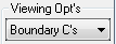 .
. - Enable editing the grid by checking Enable Edit
 (See Figure 1617)
 - RMC on the tidal location cell and select New (See Figure 2223)
- Enter the Boundary Group ID, "Ocean" (See Figure 2223)
- Select the appropriate boundary type. In this case, the river flows to the east, so choose "4" for the "Open BC:East" as shown in Figure 2223.
| Anchor | ||||
|---|---|---|---|---|
|
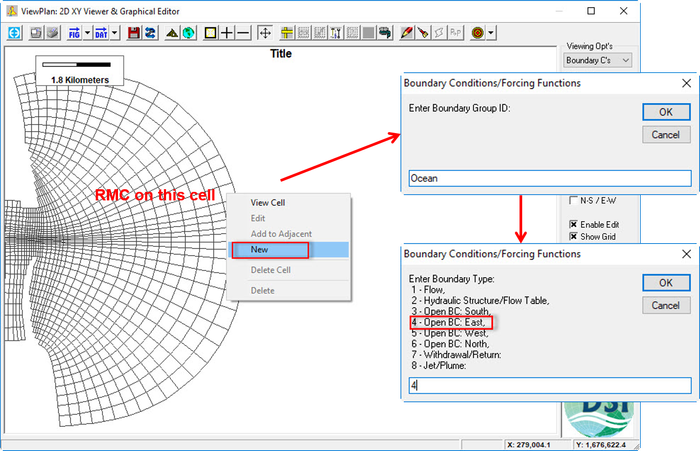
Figure 22 23 Set the tidal boundary.Anchor
7. Select the water level time series that created earlier, "Tides" as shown in Figure 2524.
| Anchor | ||||
|---|---|---|---|---|
|

Figure 25 24 Assign tides boundary.
9. The open boundary often contains a lot of cells so it is not convenient to use the feature of Add to Adjacent cells that was used when we assigned the inflow boundary. In order to select multiple cells, we can to draw a line across all the cells as open boundaries. Then, click to Add by Polygon button (Figure 2524).
10. Browse to "Open_BC Line.p2d" in Data folder then click Apply and then OK button. (See Figure 2625).
11. Click Set All button in Figure 2524 to assign tides to all cells.
12. The tides is now assigned to all open BC cells. (See Figure 2726).
| Anchor | ||||
|---|---|---|---|---|
|
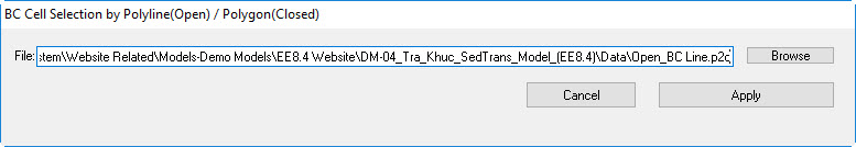
Figure 26 25 Selecting multiple BC cells by polyline/polygon.
| Anchor | ||||
|---|---|---|---|---|
|
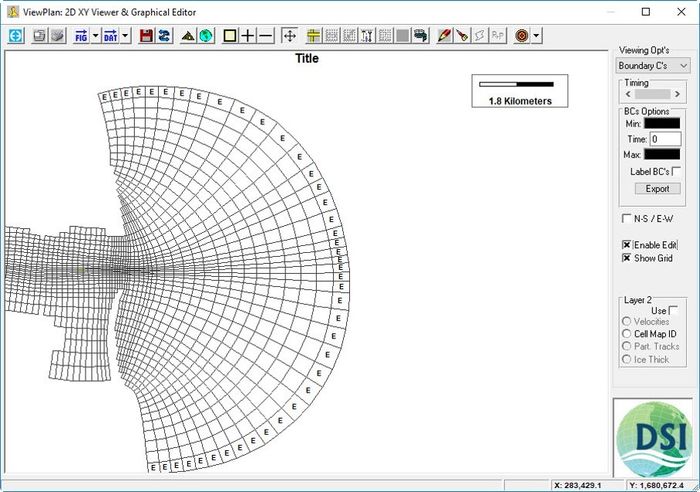
Figure 27 26 Tidal BC cells assigned.
| Anchor | ||||
|---|---|---|---|---|
|
In order to optimize simulation time, the EFDC model can be set so that dry cells are ignored with Wetting and Drying frame. In this case we should set this condition as following:
- Select Hydrodynamics/ Wetting & Drying box
- Set Flag is equal to -99.
- Entering the Wet/Dry Depth. Remember that the wet depth should always greater than the dry depth. (Figure 2827).
| Anchor | ||||
|---|---|---|---|---|
|
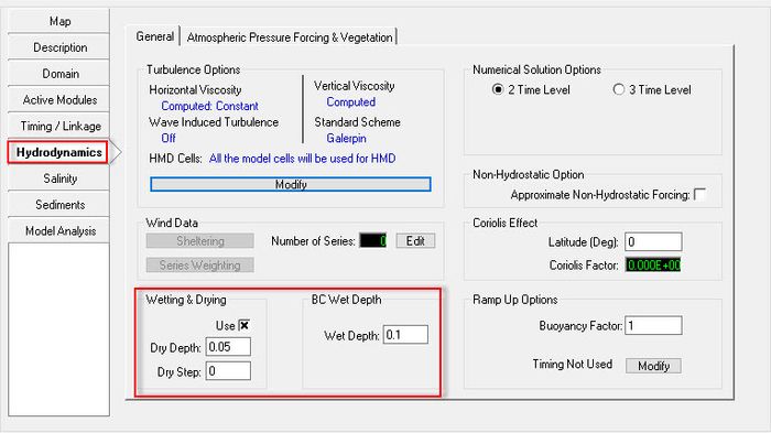
Figure 28 27 Hydrodynamic Model Setup.
4. Click Modify button in Turbulence Options to set turbulence diffusion ( See Figure 2928)
| Anchor | ||||
|---|---|---|---|---|
|
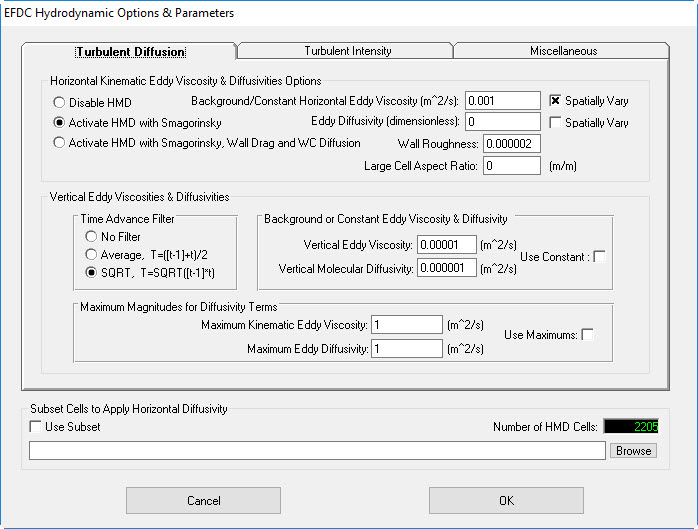
Figure 29 28 Turbulence Diffusion Settings.
...
| Anchor | ||||
|---|---|---|---|---|
|
The hydrodynamic model is ready for running test now. Normally a model is run for one vertical layer for initial calibration and more vertical layers are added later. To increase the number of vertical layers:
- Open the Domain/ Grid tab and enter the number of vertical layers into the box as in this case the vertical layers are equal to 5 layers. (Figure 3029).
- Save the model project.
| Anchor | ||||
|---|---|---|---|---|
|
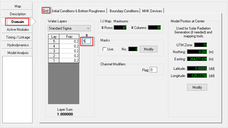
Figure 30 29 Setting the Vertical Layers.
| Anchor | ||||
|---|---|---|---|---|
|
We have now almost completed the hydrodynamic model. The final step is to set the model simulation time and model time steps.
- Select Timing/ Linkage and Model Run Timing (Figure 2827)
- Enter duration of starting/ ending the simulation. Note that the boundaries time series should be always covered this simulation duration period. Otherwise the model will not run.
| Anchor | ||||
|---|---|---|---|---|
|
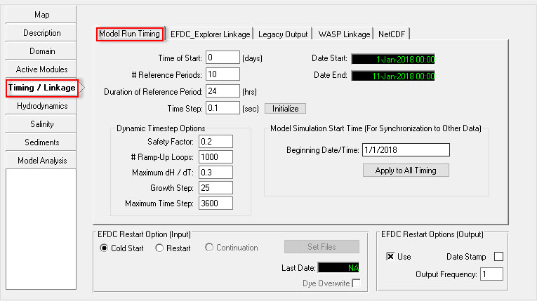
Figure 31 30 Setting the model run time.
3. Select the EFDC_Explorer Linkage tab to set the frequency of the output of the EFDC results. Setting this to 60 minutes means that EFDC will save the output every 15 minutes for display of the model results in the EE. (Figure 3231). Note that, smaller output frequency will create a larger output file.
| Anchor | ||||
|---|---|---|---|---|
|
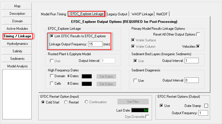
Figure 32 31 Setting Linkage Output Frequency.
| Anchor | ||||
|---|---|---|---|---|
|
| Anchor | ||||
|---|---|---|---|---|
|
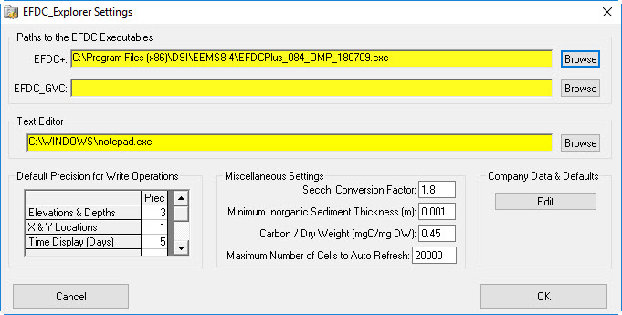
Figure 33 32 Browse to the EFDC executable file.
2. Select the Run EFDC icon to  on the main form and click the Run EFDC+ button to run the model (Figure 3433).
| Anchor | ||||
|---|---|---|---|---|
|
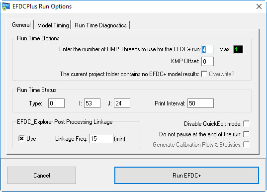
Figure 34 33 Run EFDC settings.
If you have correctly followed this example the model will start running and you will see the MS-DOS Window appear to shown the model results as see in Figure 3534. Note that you can hit any characters on the keyboard to pause the simulation and check the model results. If you want to exit the simulation hit the same key, if you want to continue run then hit any other key.
| Anchor | ||||
|---|---|---|---|---|
|
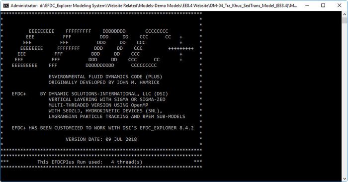
Figure 35 34 Running EFDC Window.
| Anchor | ||||
|---|---|---|---|---|
|
...
- Select the ViewPlan button.
- Scroll drown the Viewing Opt’s to choose the parameters that you want to view the model results. Figure 3635 is an example of showing the vector and magnitude velocity field results. Similarly, you can select other parameter to show the results.
- RMC on to the legend scale to access the ViewPlan Display Options (Figure 3736).
| Anchor | ||||
|---|---|---|---|---|
|
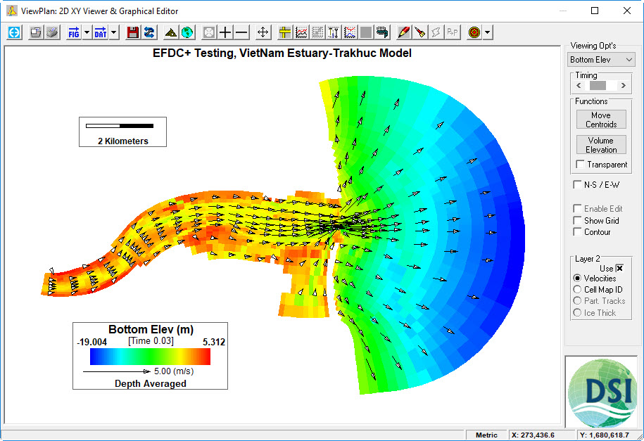
Figure 36 35 Visualizing the EFDC+ solution.
| Anchor | ||||
|---|---|---|---|---|
|
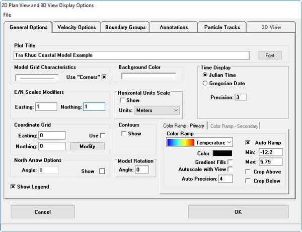
Figure 37 36 ViewPlan Display Options.
...
There are few main features in the Toolbar that are very often used when analyzing the model results. Explanations for these buttons provided in Table 1 below.
| Anchor | ||||
|---|---|---|---|---|
|
...