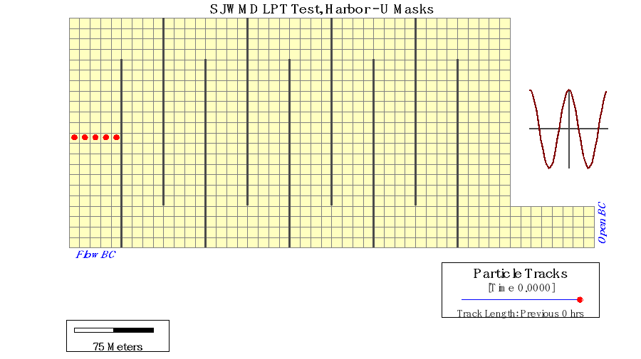
An example of the LPT function may be seen in Figure 1. This example consists of a rectangular domain with flat bottom, an open boundary to the east and a flow boundary along the southwest edge. U component masks were inserted to demonstrate the functionality of the Lagrangian Particle Tracks computations when masks are used.
| Anchor | ||||
|---|---|---|---|---|
|
Figure 1 Harbor_U grid showing the masks, boundaries and initial particle locations.
...
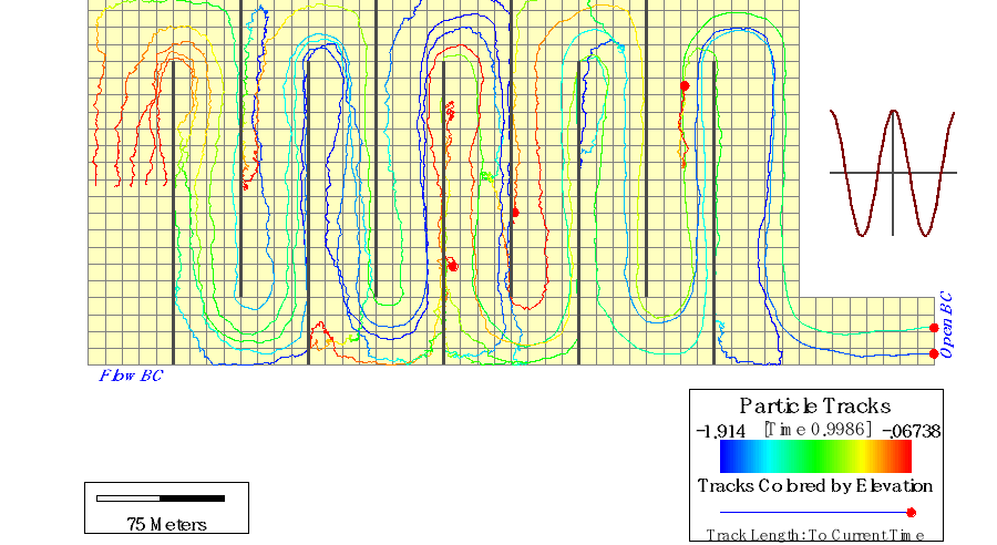
Figure 3 shows the particle tracks colored by elevation and with random walk applied. Even though there was no vertical component, the tidal range is seen to result in changing particle elevations.
...
| Anchor | ||||
|---|---|---|---|---|
|
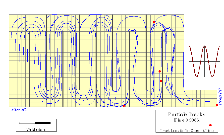
Figure 2 Harbor_U: Trajectories of 5 drifters over 1 day (no random walk).
| Anchor | ||||
|---|---|---|---|---|
|
Figure 3 Harbor_U: Trajectories of 5 drifters over 1 day (random walk).