Downstream Projection for velocity feature (available from EEMS10.4) allows the user to specify an orientation angle (degrees clockwise from north, looking downstream) in order to plot the velocity magnitude of upstream and downstream flow during the EE data extraction.It is accessed by RMC when in the Velocities viewing option as shown in Figure 3.of a given cell over a user-defined period of time.
This feature is available from the 2DH View, from which a velocity layer must be added and the active mode turned on in the Layer Control as presented in Figure 1. The user is then able to select a location of interest and the information of the selected cell will be presented in a yellow box.This feature allows the user to specify an orientation angle (degrees clockwise from north, looking downstream) in order to plot velocity magnitude of upstream and downstream flow during the EE data extraction. It is accessed by RMC when in the Velocities viewing option as shown in Figure 3.
If the user has selected All Layers in the Layer Settings then the user can optionally plot the average current velocity for the water column entirely or partly. This feature is primarily used when an exact comparison of model results with measured data is required in cases where the depth below the surface of the measuring device is known. For the settings RMC on the selected cell and click Downstream Projection (as shown in Figure 5 EE will produce the plot shown in Figure 6 for all layers. 1). Use the form shown in Figure 2 to select the times to plot within the range of the whole model time (provided at the top of the form). Please note that the time format is presented in Julian date format.
From (%) is used to indicate the percentage of the water column to be displayed from the bottom of the water column up to the To (%). For example, in a 10 m water column, from 10% to 90% means the velocity magnitude it will be plotted from 1 m above the bottom and up to 9 m from the bottom.
Finally, click the OK button to start extracting and the result is shown in Figure 3.
Anchor Figure 1 Figure 1

Figure 1. The Velocity layer.
Anchor Figure 2 Figure 2
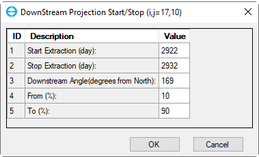
Figure 2. Select Times to Plot. Time Series – Velocity Orientation Output.
Anchor Figure 3 Figure 3
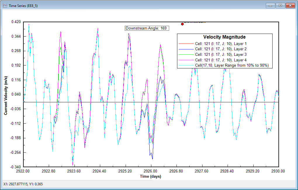
Figure 3. Velocity Projection Plot for the selected cell with all layers.