This guidance is based on the assumption the user has a correctly configured and running EFDC+ hydrodynamic and temperature model. From this model the user will be guided on how to configure EEMS to export the required files for WASP7/8 water quality simulations. The model used in this example can be run in demo mode of EEMS, and may be downloaded from here.
Generate WASP linkage file (*.hyd) from EFDC+
The first step is to generate a hydrodynamic linkage file (*.hyd) for use in the WASP model. From the Model Control form, go to the Timing/Linkage tab, as shown in 2085912617.
| Anchor | ||||
|---|---|---|---|---|
|

Figure 1. WASP Linkage Output Setting from EE.
From Timing/Linkage tab:
(1) RMC on Linkages sub-tab;
(2) From EFDC Model Linkages form, go to WASP Linkage tab;
(3) Select WASP radial under Linkage to Water Quality Model frame, then select WASP8HYDRO from the drop-down list;
(4) Type in 10 to Number of Minutes to Average per Linkage Step box to set the output frequency of the linkage file. In this case, the wasp linkage output will be saved per 10 minutes.
(5) Click OK button to save the setting
In the model interface, click on Save to save the model, as shown in 2085912617, below.
| Anchor | ||||
|---|---|---|---|---|
|
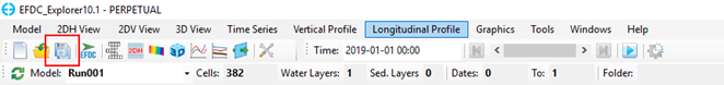
Figure 2. Save Button in the Model Interface.
After clicking on the Save button, a Select Directory: Write Operation a pop-up will appear to select saving options (refer to 2085912617). Before project files are saved, the grey box is empty. This is where EE project files will be listed. The empty gray box shows that no files have been written yet for the study, as shown in 2085912617.
Three save options are offered in the Save Options frame of 2085912617:
- Full Write can be selected to save all the input files,
- Write All except Time Series Files can be selected to save all input files without the time series.
- Save Profile File Only (EFDC.EE) can be selected for saving if the user has only changed formatting options in EE.
In this project, the Full Write option is recommended. After choosing this option, click OK to close the form and save the model.
| Anchor | ||||
|---|---|---|---|---|
|
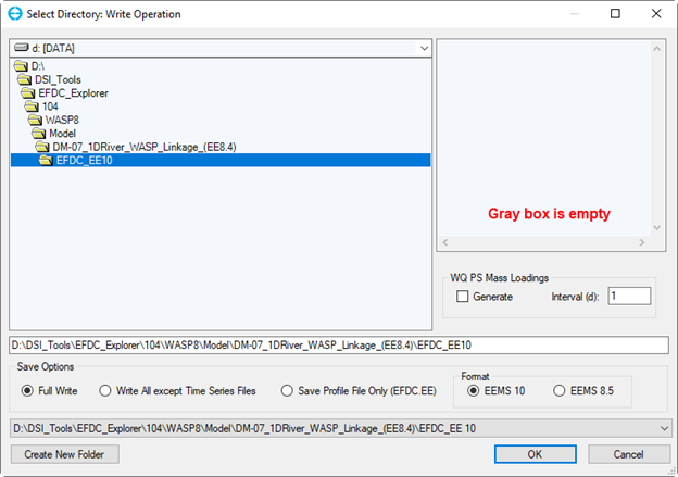
Figure 3. Saving the model.
To run the model, follow the steps below, as shown in 2085912617.
Click on the Run EFDC+ button at the top of the model interface to run the model. The EFDC+ Run Options form will appear; 2085912617. in this form, under the General tab, set the Number of OMP Threads to use for the EFDC+ run in the EFDC+ Multi-Threading frame. Note that the number of threads used for the EFDC+ run must be smaller than the total number of threads.
Also, in the EFDC+ Multi-Threading frame set the KMP Offset to set the threads that will be passed over when running the model. For example, if KMP Offset is set to 2, which means the thread used for the EFDC+ run will start from the 3rd thread. This can be used to run multiple models on one machine, so the models run on different threads.
Note: If the model has existing results, please check the Overwrite check box to run and save new results.
| Anchor | ||||
|---|---|---|---|---|
|
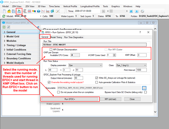
Figure 4. EFDC+ Run Options form.
Click on the Run EFDC+ button to start running the model. A run window such as that pictured in 2085912617 will appear.
| Anchor | ||||
|---|---|---|---|---|
|
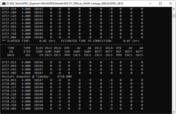
Figure 5. EFDC+ run window.
After the EFDC+ model run is finished, the user should browse to the output folder to make sure that the efdc_dsi_wasp.hyd file has been generated. It should be noted that the WASP8SEG_EFDCIJK.DAT file allows the identification of the corresponding segment between the WASP and the EFDC cell.
| Anchor | ||||
|---|---|---|---|---|
|

Figure 6. WASP Linkage file generated by EFDC+.
Building WASP model with using Hydrodynamics Linkage
From the WASP program interface, click on the New button in the toolbars to create a new project
| Anchor | ||||
|---|---|---|---|---|
|
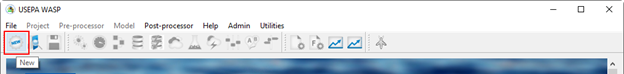
Figure 7. Create a new WASP project.
After creating a new project, click on the Data Set button, which is now enabled in the toolbar, then carry out the following steps to link hydrodynamic input:
(1) Check on Hydrodynamics checkbox, then browse to the efdc_dsi_wasp.hyd file generated from EFDC+;
(2) Select the Solution Technique as Cosmic ;
(3) Modify the Model Output Interval for the output frequency;
(4) Click the OK button to save the setting (2085912617).
| Anchor | ||||
|---|---|---|---|---|
|
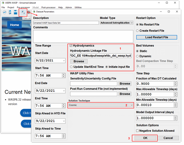
Figure 8. Link hydrodynamics output from EFDC+ to WASP model.
The next step when setting up a new WASP is to check at this point if the data provided by EFDC+ hydrodynamic linkage file are read correctly by WASP8. User can also check the numerical stability of the hydrodynamic linkage by inspecting the “Mass Check” system on the runtime and in model output.
For WASP 8 the output is not turned on automatically, so the user must go to the Output Control button from the toolbar to select the output parameters that will be written out.
(1) Click on the Output Control button from the toolbar
(2) Check on the output checkboxes for Mass Check, as well as the transport quantities that user wants to write out to compare with the EFDC+ model.
(3) Click the OK button to save the setting (2085912617).
| Anchor | ||||
|---|---|---|---|---|
|
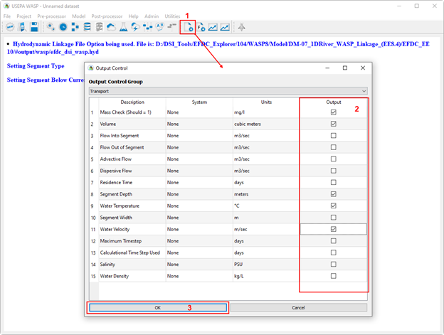
Figure 9. Select WASP output parameter to write out.
In the model interface, click on the Save button to save the model, as shown in 2085912617 below.
| Anchor | ||||
|---|---|---|---|---|
|
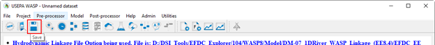
Figure 10. Save Button in the Model Interface.
After the model has been saved, the Executable button will now be enabled. Click on the Executable button to start run the WASP model, and the runtime simulation interface will be displayed as shown in 2085912617 below.
| Anchor | ||||
|---|---|---|---|---|
|
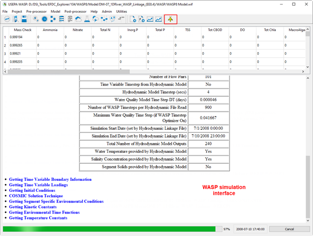
Figure 11. WASP model run interface.
Wait until the model run finishes, then click on the WRDB Graph button from the toolbar for the post-processing.

The WRDB Graph window now appears, from the WRDB Graph window,
(1) Click the Open button from the toolbars
(2) Browse to the WASP output file (*.BMD2)
(3) Click the OK button (2085912617).
| Anchor | ||||
|---|---|---|---|---|
|

Figure 12. Open WASP output from WRDB Graph.
After the Manage Data Series form is displayed:
(1) Select the output file that the user wants to extract
(2) Select the segment (cell index in EE) from which the user wants to extract output
(3) Select the parameters for which the user wants to extract output. In this case, we select Mass Check and Water Velocity as the parameter to plot
(4) Click on the Add to Left/Right Axis buttons to add the series to the left Y-axis or right Y-axis
(5) The extracted data series will be listed here
(6) Click the Close button to close the form and plot the output series (2085912617).
| Anchor | ||||
|---|---|---|---|---|
|
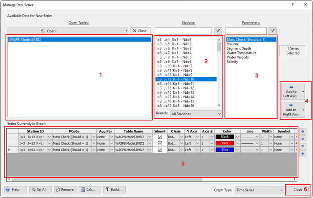
Figure 13. Manage data series to plot.
The mass check data time series will be plotted as shown in 2085912617 below.
| Anchor | ||||
|---|---|---|---|---|
|
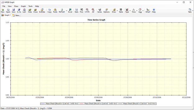
Figure 14. Data series plotted by WRDB Graph.
As shown in 2085912617, the mass check concentration of the segments approaches 1
...
.0 mg/L. It means the simulation is run for a sufficient duration and reaches steady-state.
2085912617 shows a comparison of the water velocity in WASP and EFDC+ at cell yy. The two curves are almost identical, provide verification of the flow information from the hydrodynamic linkage.
| Anchor | ||||
|---|---|---|---|---|
|
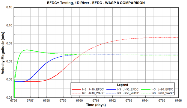
Figure 15. EFDC+ and WASP 8 velocity Comparison.
Building WASP water quality model
From the WASP interface,
(1) From toolbars, go to Pre-processor\Systems
(2) Click the Insert button to add the water quality constituents that the user wants to simulate
(3) Click on the drop-down list in each row under the System Type column to set the water quality constituent. The user can also define a more familiar name for water quality constituents under the System Name column
(4) Click the OK button to save settings (2085912617)
| Anchor | ||||
|---|---|---|---|---|
|
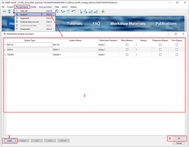
Figure 16. Add water quality constituents to the WASP model.
After adding water quality constituents to the WASP model, we will now add the boundary condition in the next step. From the WASP interface, go to Pre-processor\Boundary Condition and Loads as shown in 2085912617 below.
| Anchor | ||||
|---|---|---|---|---|
|
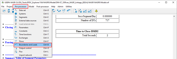
Figure 17. Add water quality boundary conditions to WASP model.
From Boundaries and Loads form, under Boundaries tab
(1) Select the cell corresponding to each boundary and constituent;
(2) Fill in the data series for the selected constituent;
(3) After filling the data series for all boundaries, click OK to save the boundary data (2085912617).
| Anchor | ||||
|---|---|---|---|---|
|
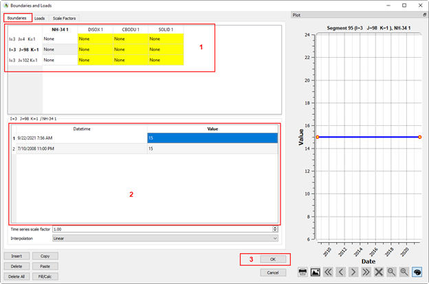
Figure 18. Add water quality boundary conditions data series.
After the boundary conditions have been added, we will set the model parameters and kinetic coefficients for the model.
From the WASP interface, go to Pre-processor\Constants as shown in 2085912617.
| Anchor | ||||
|---|---|---|---|---|
|
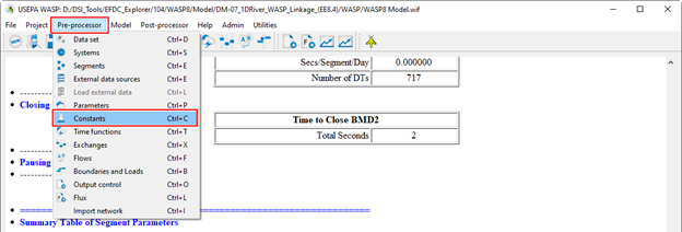
Figure 19. Set model parameters and kinetic coefficients.
From Constants form,
(1) Select the constant group;
(2) Check on the checkbox corresponding to the parameter that will be used to simulate in the model;
(3) Set the parameter values for constant groups as shown in 2085912617 to 2085912617;
| Anchor | ||||
|---|---|---|---|---|
|
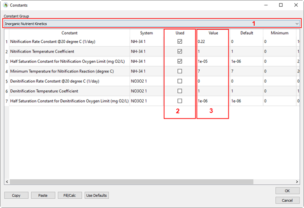
Figure 20. Set Inorganic Nutrient kinetics parameters.
| Anchor | ||||
|---|---|---|---|---|
|
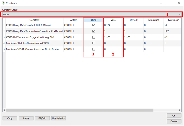
Figure 21. Set CBOD parameters.
| Anchor | ||||
|---|---|---|---|---|
|
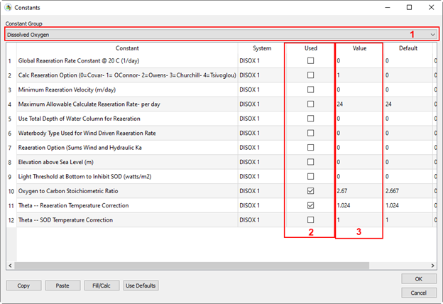
Figure 22. Set dissolved oxygen parameters.
| Anchor | ||||
|---|---|---|---|---|
|
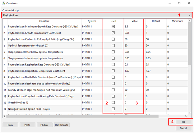
Figure 23. Set Phytoplankton parameters.
(4) Click OK button to save settings after set the kinetic parameters as shown in 2085912617;
After set the model parameters, from toolbar, click on the Output Control button to open Output Control form and add the water quality constituents to the output as shown in 2085912617.
| Anchor | ||||
|---|---|---|---|---|
|

Figure 24. Set Output Control.
From the Output Control form,
(1) Select the Output Control Group;
(2) Check on the checkbox corresponding to the parameter will be written out as shown in 2085912617 to 2085912617;
| Anchor | ||||
|---|---|---|---|---|
|
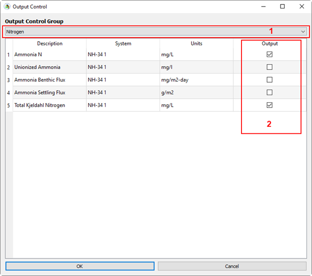
Figure 25. Add Nitrogen parameters to the output.
| Anchor | ||||
|---|---|---|---|---|
|
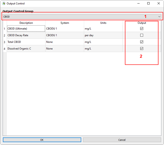
Figure 26. Add CBOD parameters to the output.
| Anchor | ||||
|---|---|---|---|---|
|
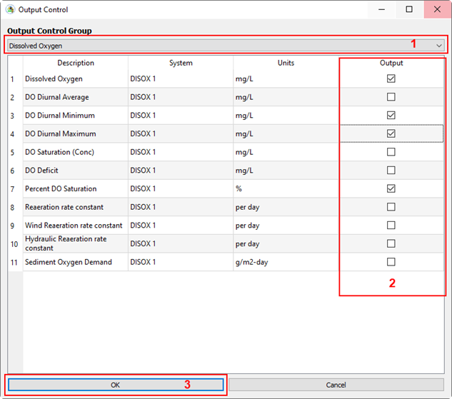
Figure 27. Add DO parameters to the output.
(3) Click the OK button to save settings as shown in 2085912617;
After finishing the settings for the model, from the toolbar,
- Save the model;
- Run WASP model as shown in 2085912617
| Anchor | ||||
|---|---|---|---|---|
|

Figure 28. Save and run WASP model.
Visualize WASP Output
Wait for the model run finish, then go to WRDB Graph to check the model output as we did for checking hydrodynamics output before.

The WRDB Graph window now appears, from WRDB Graph window,
(1) Click the Open button from the toolbars
(2) Browse to the WASP output file (*.BMD2)
(3) Click the OK button (Open WASP output from WRDB Graph 2085912617).
| Anchor | ||||
|---|---|---|---|---|
|
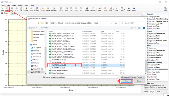
Figure 29. Open WASP output from WRDB Graph.
Manage Data Series form appears, from here
(1) Select the output file that the user wants to extract
(2) Select the segment (cell index in EE) that the user wants to extract output
(3) Select parameter that user want to extract output
(4) Click on Add to Left/Right Axis buttons to add the series to the left Y-axis or right Y-axis
(5) The extracted data series will be listed here
(6) Click the Close button to close the form and visualize the output series (2085912617).
| Anchor | ||||
|---|---|---|---|---|
|
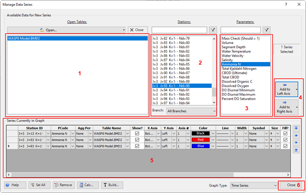
Figure 30. Manage data series to plot.
The data series will be plotted as shown in 2085912617 below.
| Anchor | ||||
|---|---|---|---|---|
|
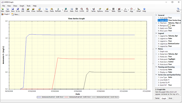
Figure 31. Data series plotted by WRDB Graph.
Note: In the bottom right corner of the Manage Data Series form, the Graph Type frame is available to allow the user to view the output in different ways, as shown in 2085912617 below.
| Anchor | ||||
|---|---|---|---|---|
|
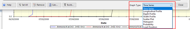
Figure 32. Graph type of WRDB Graph.
For graph types like Longitudinal Profile, Depth Profile, for which the value change by time, the timing bar is available in the bottom of the WRDB Graph window (2085912617). Therefore, the user can move the time or run animation to see how the output changes in a profile.
| Anchor | ||||
|---|---|---|---|---|
|
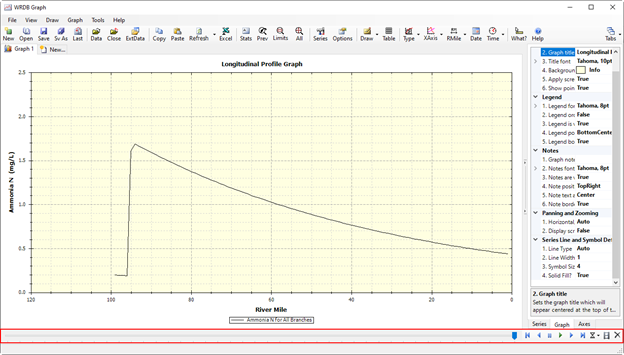
Figure 33. Timing bar in Longitudinal Profile Graph.
After the output graphs have been plotted, from toolbars, the user can select Send data and graph to Microsoft Excel button to extract data then import as external data to EE to compare the output between WASP and EFDC+.
Some output comparison graphs are shown in 2085912617 to 2085912617 below.
| Anchor | ||||
|---|---|---|---|---|
|

Figure 34. Time series comparison of water temperature between EFDC+ and WASP output.
| Anchor | ||||
|---|---|---|---|---|
|

Figure 35. Time series comparison of DO between EFDC+ and WASP output.
| Anchor | ||||
|---|---|---|---|---|
|
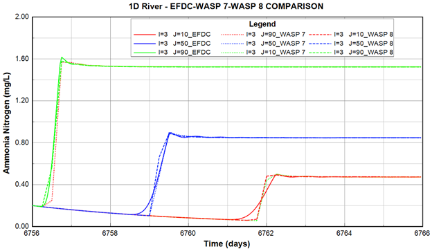
Figure 36. Time series comparison of NH3-N between EFDC+ and WASP output.
| Anchor | ||||
|---|---|---|---|---|
|
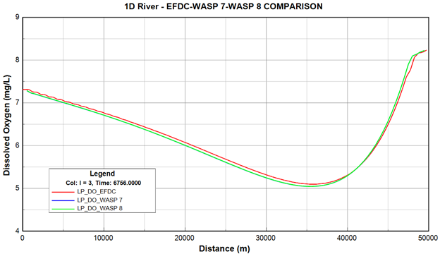
Figure 37. Longitudinal profile comparison of DO between EFDC+ and WASP output.
| Anchor | ||||
|---|---|---|---|---|
|
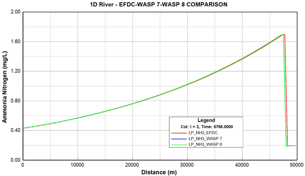
Figure 38. Longitudinal profile comparison of NH3-N between EFDC+ and WASP output.