The user may select which parameters are to be displayed by accessing the Data Series form by RMC’ing on the legend or select Format Data Series from the toolbar. An example of the form is shown in Figure 1.
| Anchor | ||||
|---|---|---|---|---|
|
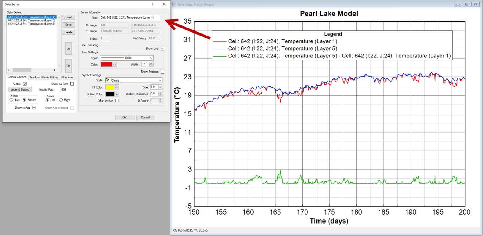
Figure 1. Data Series form.
...
The lines available for viewing are displayed on the left in the Data Series box ( as shown in Figure 2).
The series formatting and axes formatting can be saved for later retrieval using the Save and Load buttons. The Delete button will delete the series selected (highlighted) in the Data Series frame (left-hand box).
...
The right side of the form is the Series Information frame ( as Figure 3) that shows the maximum and minimum values, and the number of points for the selected line. The legend text for the selected line can also be changed in this frame. In the Line Formatting frame, the user may set thickness, color, and style with the drop-down menus.
...
Figure 3. Series information.
General Options
Figure 4 show the General Options frame, that the user can toggle the display of each line by checking Visible for the series selected. An extra Y-axes can be added to the right of the graph by setting the Right tab in the “Y-Axis” subframe. Other features include changing lines to bar graphs with the “Show as Bars” check box.
...
The Transform/Series Editing tab in Figure 5 provides options for the user to adjust the data with additive and multiplicative adjustment factors for both the X and Y component for plotting purposes. The form also provides a means to add or subtract one series from another and place the resultant series into a specified series with the Add/Subtract Series button. The edited data does not update the EFDC data directly. If desired, an edited series can be exported from the time-series plot and used to update the model input data.
...
In the Filer lines, the user can choose any time series to filter as shown in Figure 6. After Apply Filter is selected a new time series will be plotted with its filtered series, an example of which is shown in Figure 7.
| Anchor | ||||
|---|---|---|---|---|
|
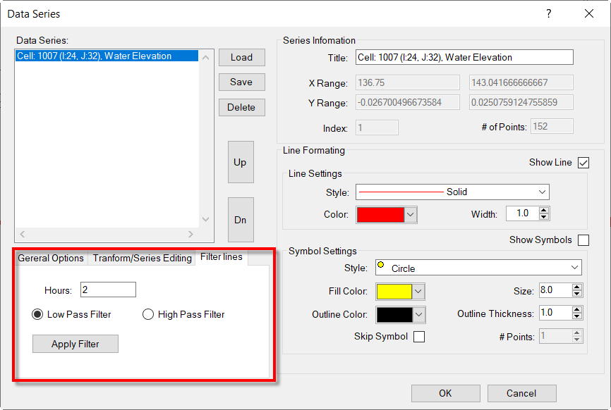
Figure 6. High and Low Pass Filter for Time Series Plotting.
| Anchor | ||||
|---|---|---|---|---|
|
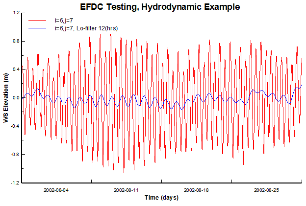
Figure 7. Time Series plot of WSEL (red) and low pass filter (blue) at location i=6, j=7.
Interval
The Interval tab in Figure 8 provides options for the user to adjust the time period between data points in the plot.
For example, Figure 9 presents the time series of the velocity magnitude from the model output with a 1-minute interval, therefore there is a gap line when the data is missing. When the user uses the interval options and selects the interval greater than the previous one, the missing data can be removed as shown in Figure 10. In the Interval tab, click Use Interval (days) checkbox, select the interval and then click Apply. The model interval and the number of data points are summarized in the box. When plotting data time series which has gaps (missing data), the plot will have a straight line, as shown in Figure 9. To remove that straight line, the Gap tab in the Data Series form as shown in Figure 8 can be used. Select the Gap, EE will calculate the data gap and number of data points in the underneath table; the gap is presented in hours. Based on the data gap, the user can enter a value that should be greater than the gap in the box Maximum Gap (hours), click Use checkbox, next click Apply button. Then click the OK button, the plot without the straight line is shown as Figure 10.
| Anchor | ||||
|---|---|---|---|---|
|
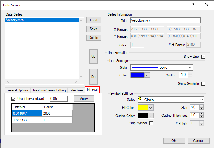
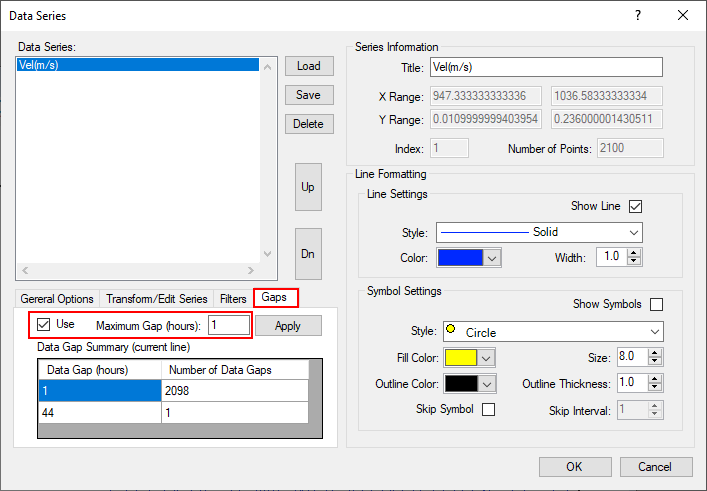
Figure 8. Interval options.
...
Figure 9. The time series plot before applying intervalsthe interval option.
Anchor Figure 10 Figure 10
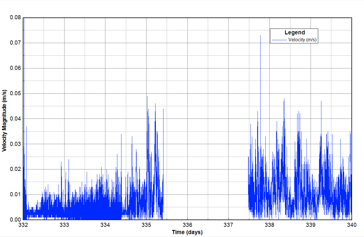
Figure 10. The time series plot after applying intervalsthe interval option.