...
Figure 38- After clicking “New “ the pre-processor button is now ready to import the EFDC HYD file.
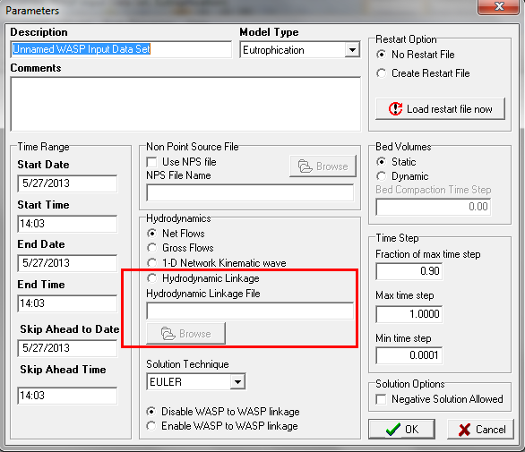
Figure 39- When you click on Pre-Processor, this screen is opened.
...
Figure 43- Data read from EFDC HYD file for the 1D river problem, page 1 of 2.
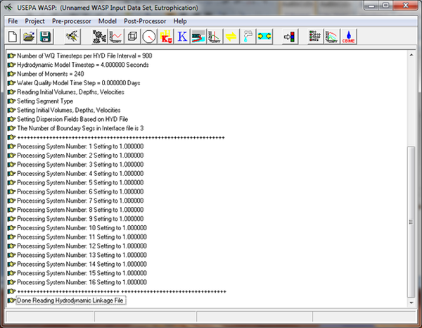
Figure 44- Data read from EFDC HYD file for the 1D river problem, page 2 of 2.
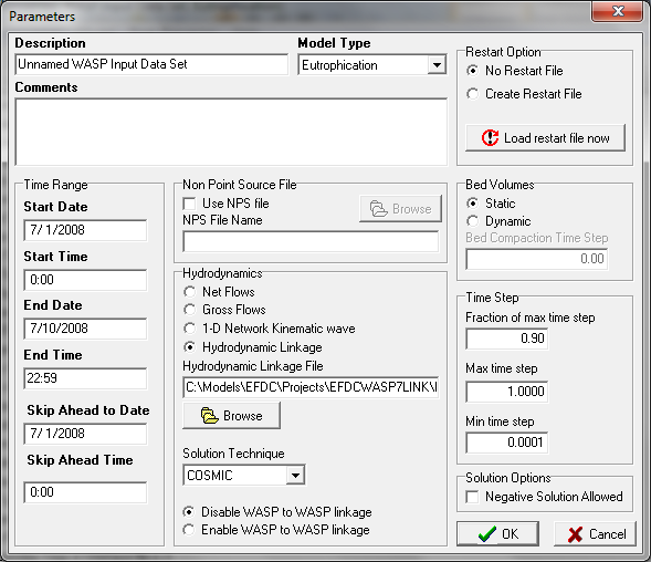
Figure 45- Pre-processor page beginning and ending date and time.
...
Go back to “File” button on main screen and click ‘Save As’ project file, then you use browser to save the WASP7 project file to the folder for WASP7 projects (not EFDC projects).

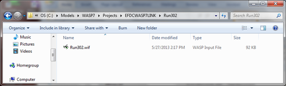
Figure 46- WASP7 project file saved in WASP7 project folder (not the EFDC project folder).
The next set of steps in setting up the WASP7 project is the input of boundary condition data for each state variable and each boundary segment. Screenshots shown in Figure 47 through Figure 56 show the assignment of default boundary condition data and testing the boundary condition settings for the 1D river problem.
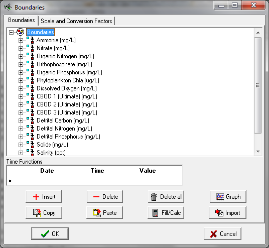
Figure 47- Pre-Processor Selection for Boundaries brings up this screen after you click on (+) sign for Boundaries.
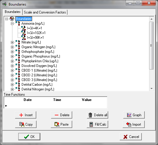
Figure 48- Click on Ammonia (+) and list of boundary segments is displayed.
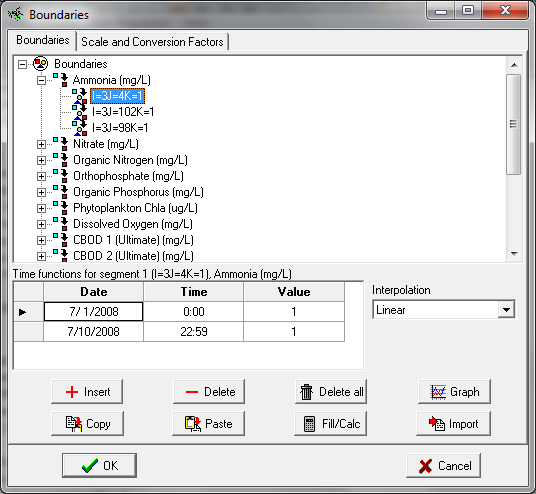
Figure 49- Default boundary settings for Ammonia.
Click on segment I=3 J=4 K=1 (which is downstream boundary segment) and the default setting of 1.0 for boundary condition data is displayed in the Time Function screen. Ammonia boundary value of 1.0 is set for begin date/time 7/1/2008 00:00 and end date/time 7/10/2008 22:59.
WASP7 assigns a default setting of 1.0 for all boundary conditions for all state variables. WASP7 boundary segments are setup with linkage data for EFDC grid cell model domain.
When setting up a new WASP7 project, EPA recommends that a model run be executed at this point to test that the data provided by EFDC hydrodynamic linkage will result in a stable WASP7 model solution.
Next step is to go to main screen and execute the WASP7 model to test the boundary settings of 1.0.
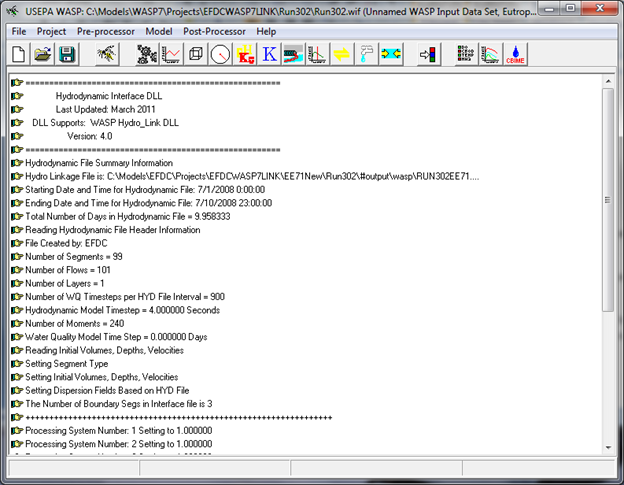
Figure 50- Click on Model and execute WASP7.
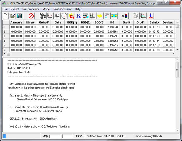
Figure 51- Screen display when WASP7 is executing.
Estimate of time remaining for WASP7 model run is shown at lower right of screen.
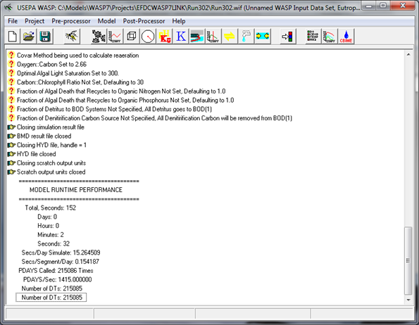
Figure 52- WASP7 run has completed successfully.
Next check the simulation results to see if model has converged to steady state solution of 1.0 mg/L at a selected grid segment. Click on Post-processor to extract time series of model results.
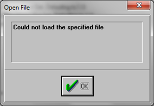
Message pops up; click OK and select the *.BMD file as the output results file for the WASP7 model
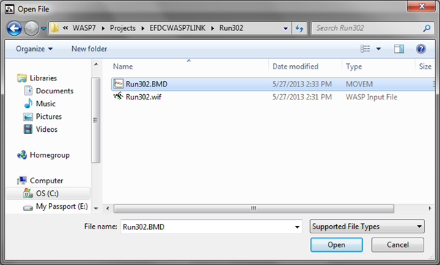
Figure 53- Select BMD file for post-processing time series results.
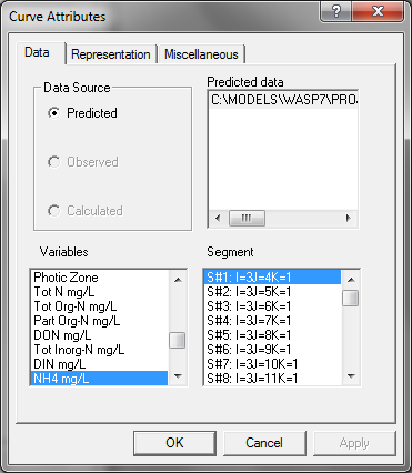
Figure 54-Select NH4 for viewing in S#1 I=3 J=4 K=1.
This is downstream boundary segment.
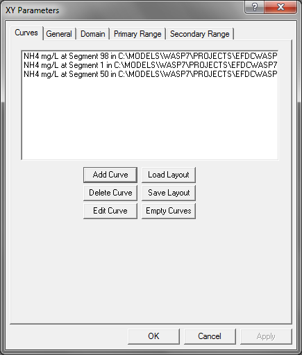
Figure 55- Select additional segments to show NH4 time series at 3 segments 98, 1 and 50.
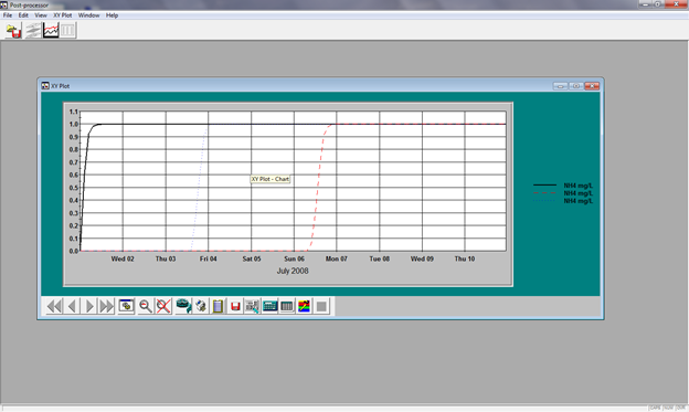
Figure 56-NH4 converges to 1.0 mg/L for 3 segments selected for display.
EFDC-WASP7 linkage is set up correctly and solution is stable.
WASP7 Boundary Condition Input for 1D River Problem
After it has been confirmed that the EFDC-WASP7 model linkage works correctly with the default boundary values of 1.0, the user must setup the actual boundary conditions and kinetic constants for each state variable for the WASP7 project. Screenshots shown in Figure 57 through Figure 61 illustrate the input of the 1D river problem boundary data to the WASP7 model.
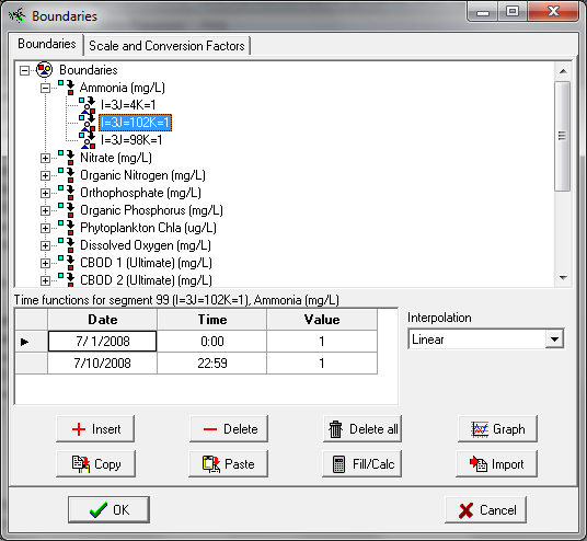
Figure 57- Boundary condition concentrations for the 1D river problem.
Boundary data for Ammonia, Nitrate, CBOD1 and Dissolved Oxygen is given in Table 1 upstream segment (I=3 J=102 K=1) and wastewater discharge segment (I=3 J=98 K=1).
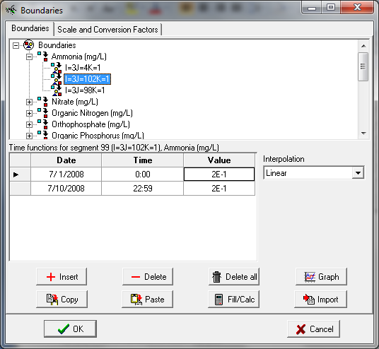
Figure 58- Upstream boundary conditions for Ammonia, NH4=0.2 mg/L.

Figure 59- Wastewater boundary conditions for Ammonia, NH4=15 mg/L.
Upstream and wastewater boundary data is assigned using the same procedure for Nitrate using boundary data from Table 1.
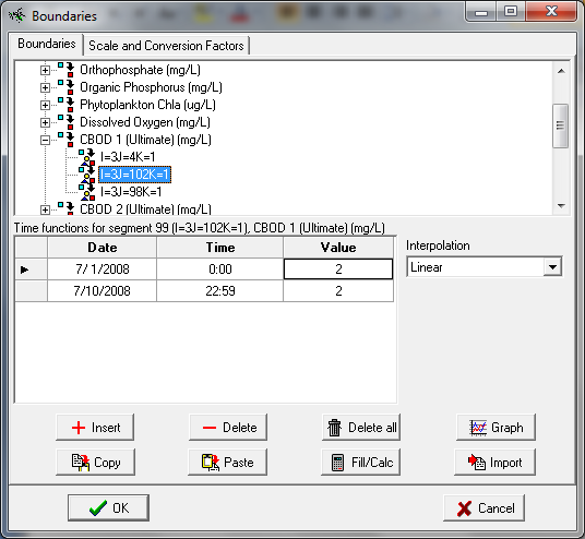
Figure 60- Upstream boundary conditions for CBOD1.
CBOD in Wasp7 is ultimate CBOD. The data given in Table 1 shows that upstream CBOD5 =1 mg/L and BOD Ultimate/5-day ratio=2 so CBOD Ultimate=2 mg/L for upstream boundary. WASP7 allows for up to 3 classes of CBOD. The 1D river problem uses only CBOD1 as the state variable for CBOD Ultimate. CBOD2 and CBOD3 are not simulated so boundary data does not have to be assigned.
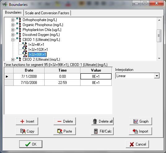
Figure 61- Wastewater boundary conditions for CBOD1.
The data given in Table 1 shows that wastewater CBOD5 =40 mg/L and BOD Ultimate/5-day ratio=2. CBOD Ultimate=80 mg/L is assigned for the wastewater boundary.
Upstream and wastewater boundary data is assigned for Dissolved Oxygen using data from Table 1. 100% oxygen saturation at Water Temperature 25 Deg-C is assigned as boundary concentration of 8.3 mg/L for upstream and wastewater discharge.
Model Parameters and Kinetic Coefficients Input for 1D River Problem
Model parameters and kinetic coefficients used for the 1D river problem are presented in Table 2. Kinetic data is input to WASP7 as ‘Constants Data’ for ammonia, nitrate, dissolved oxygen and CBOD1 as shown in the screenshots (Figure 62 to Figure 65).
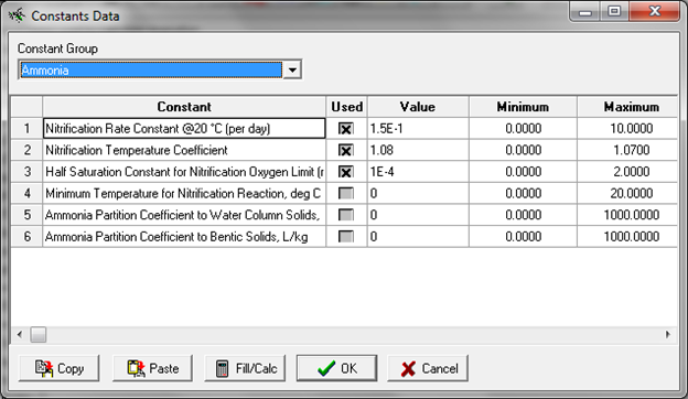
Figure 62- WASP7 Constants for Ammonia.
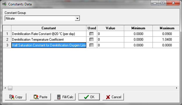
Figure 63- WASP7 Constants for Nitrate.
No nitrate constants need to be assigned for 1D rive r problem.
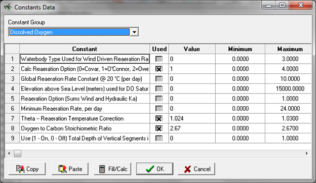
Figure 64- WASP7 Constants for Dissolved Oxygen (Reaeration Option 1=O’Connor-Dobbins).
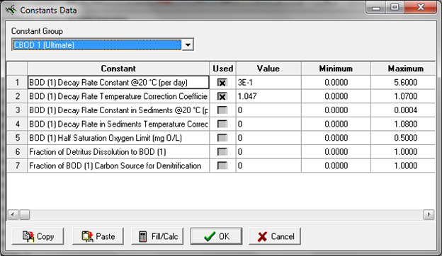
Figure 65- WASP7 Constants for CBOD1.
WASP7 Model Output and Post Processing Results
Output Control allows the user to write CSV files for selected model output variables. Data is written to CSV files as a flat data block file for all time intervals for all segments. CSV files are selected for a number of model output variables as shown in screenshots for Figure 66 to Figure 68.
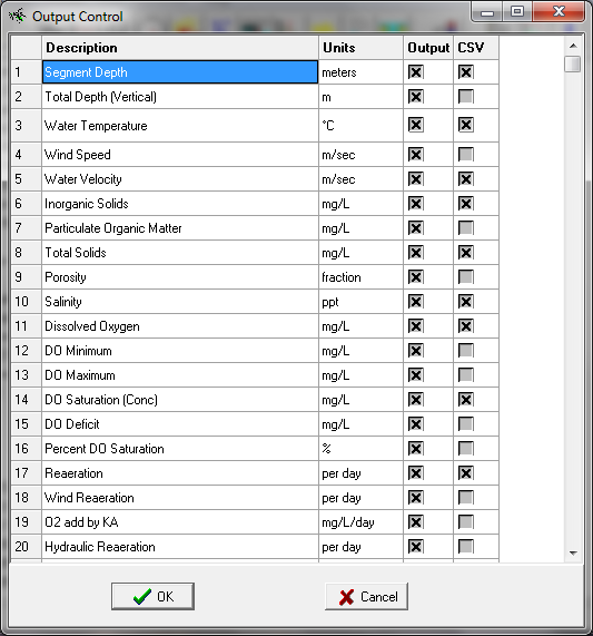
Figure 66- Output Control selection of CSV files for 1D river problem, Page 1 of 3.
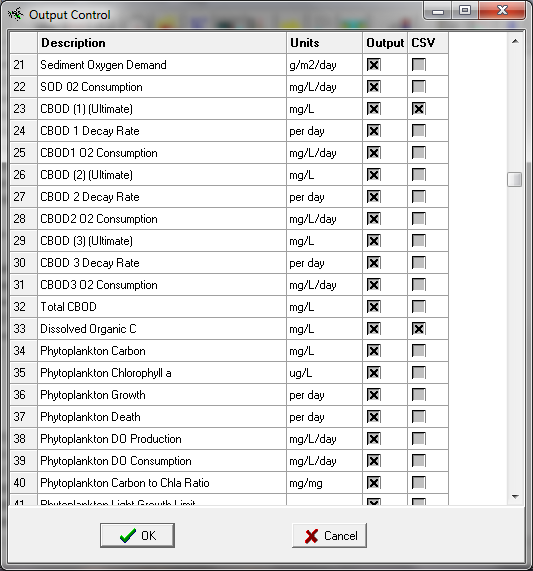
Figure 67- Output Control selection of CSV files for 1D river problem, Page 2 of 3.
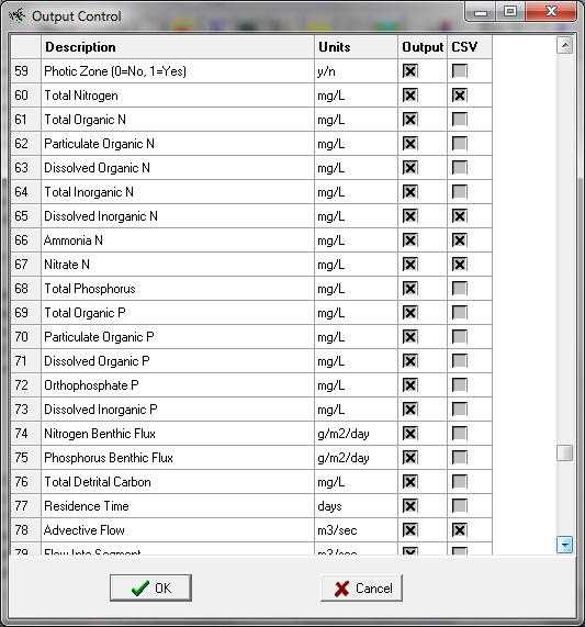
Figure 68- Output Control selection of CSV files for 1D river problem, Page 3 of 3.
Comparison of Model Results for Analytical (STREAM), EFDC and WASP7 Models
The display of steady state model results for the WASP7 model requires that a table be prepared by the user to match the WASP7 segment with a corresponding longitudinal profile x-axis coordinate for the 1D river. The upstream end of the river domain is shown in Figure 69 and the downstream end of the domain is shown in Figure 70. Model results are presented in Figure 71 through Figure 81 for depth, velocity, water temperature, salinity, CBOD5, CBODU, Total Organic Carbon (TOC), Ammonia, Nitrate, Total Nitrogen and Dissolved Oxygen.
As can be seen in the data plots, model results for both EFDC and WASP7 are in very good agreement with the analytical solution STREAM model for depth (Figure 71), velocity (Figure 72), water temperature (Figure 73), CBOD5 (Figure 75), CBODU (Figure 76), Total Organic Carbon (TOC) (Figure 77), ammonia (Figure 78), nitrate (Figure 79), Total Nitrogen (Figure 80), and dissolved oxygen (Figure 81). The good comparison of both EFDC and WASP7 with the analytical STREAM model benchmark solution confirms that the code used in EFDC and WASP7 is correct for ammonia, nitrate and dissolved oxygen state variables.
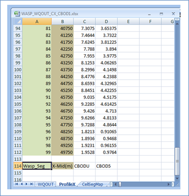 Figure 69- Data table matching Wasp7 segments with 1D river distance, upstream.
WASP Segment 99 is the upstream segment of model domain. Segment 99 extends from 50,000 to 49,500 meters. Model results plotted at midpoint of segment at 49,750 meters.
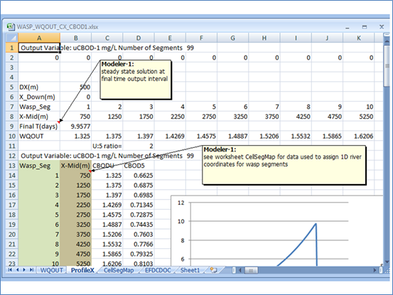
Figure 70- Data table matching Wasp7 segments with 1D river distance, downstream.
WASP Segment 1 is downstream segment of model domain. Segment 1 extends from 1000 to 500 meters. Model results plotted at midpoint of segment 1 at 750 meters. EFDC grid cell (3,3) extends from 500 to 0 meters in EFDC domain. WASP7 linkage drops downstream grid cell and assigns this cell as WASP7 segment ‘0’ boundary segment. Longitudinal profile of WASP7 steady state model results are extracted for final time interval of 9.9577 days from CSV output file data block of time and segment.
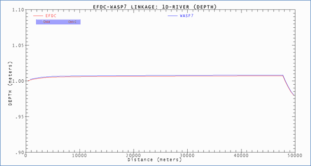
Figure 71- EFDC and WASP7 results for Stream Depth.
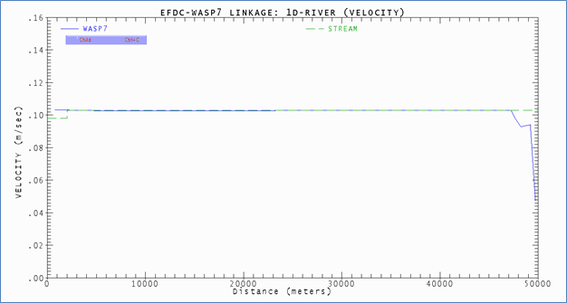
Figure 72- WASP7 and STREAM Model results for River Velocity.
Longitudinal profile of EFDC velocity is not extracted from EFDC_Explorer.
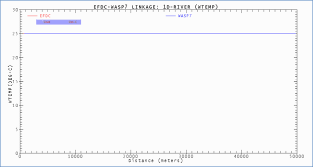
Figure 73- EFDC and WASP7 Model results for Water Temperature.
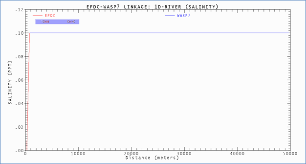
Figure 74- EFDC and WASP7 Model results for Salinity.
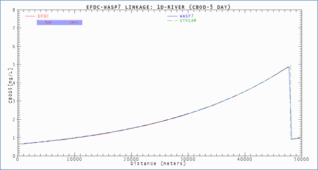
Figure 75- EFDC, STREAM and WASP7 Model results for CBOD5.
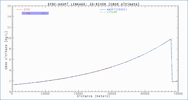
Figure 76- EFDC, STREAM and WASP7 Model results for CBOD Ultimate.
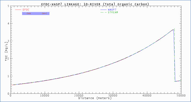
Figure 77- EFDC, STREAM and WASP7 Model results for TOC.
Note that POC=0 and TOC=DOC
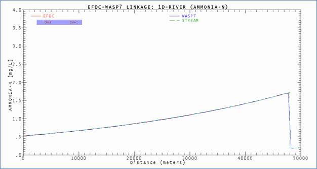
Figure 78- EFDC, STREAM and WASP7 Model results for Ammonia-N.
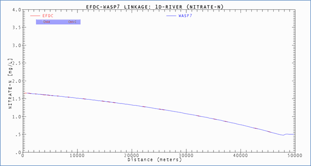
Figure 79- EFDC and WASP7 Model results for Nitrate-N.
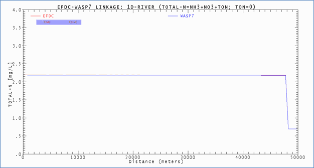
Figure 80-EFDC and WASP7 Model results for Total Nitrogen.
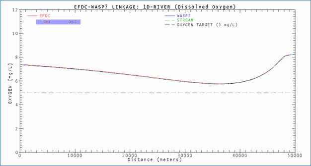
Figure 81-EFDC, STREAM and WASP7 Model results for Dissolved Oxygen.