WASP7-EFDC Linkage (1D River Example)
Introduction
This technical document provided by Dynamic Solutions International, LLC (DSI) (www.ds-intl.biz) describes the step-by-step procedures needed to create an EFDC hydrodynamic model results binary file (*.HYD) that is formatted for linkage as an input file to the WASP7 water quality model. This technical memorandum provides the information needed and example problems to show the step-by-step procedures needed to successfully create and apply an EFDC project to export a hydrodynamic file (*.HYD) for linkage as an input file for a WASP7 water quality model project. The description contained in this document assumes that the user has completed the setup of a working EFDC project for a hydrodynamic model and wishes to generate a binary HYD file as input to a WASP7 water quality model.
The user is reminded that the EFDC model and the EFDC_Explorer interface can be obtained from DSI’s EFDC_Explorer web site (www.efdc-explorer.com) includes a fully functioning coupled sediment transport and water quality model in a single EFDC model source code. The EFDC water quality model is comparable to the state variables included in the WASP7 water quality model.
Two example problems are developed by DSI to show how an EFDC model can be setup and linked to a WASP7 water quality model.
Example Problem#1. A 1D river problem for BOD, nitrogen and dissolved oxygen is setup in EFDC as a hydrodynamic, sediment transport and water quality model. The hydrodynamic results file (HYD) is then used to setup the same 1D river problem in WASP7. The results of the EFDC and WASP7 water quality models are compared to a steady state analytical model as a benchmark solution for the 1D river problem. All input files needed for the EFDC and the WASP7 models are provided for the 1D river problem.
DSI recommends using the EFDC_DSI coupled hydrodynamic and water quality model instead of the EFDC/WASP linkage process as a faster approach to water quality modeling and it provides the user with more robust tools for pre- and post-processing the water quality model. This allows the user to focus more on producing a better modeling study rather than wasting time with model/linkage mechanics.
Documentation for EFDC-WASP7 Linkage
The US Environmental Protection Agency (EPA) supports a number of public domain watershed, hydrodynamic and water quality models for use in water quality management studies including TMDL evaluations. The EPA Watershed & Water Quality Modeling Technical Support Center is the portal for downloading EPA supported models ( http://www.epa.gov/athens/wwqtsc/index.html).
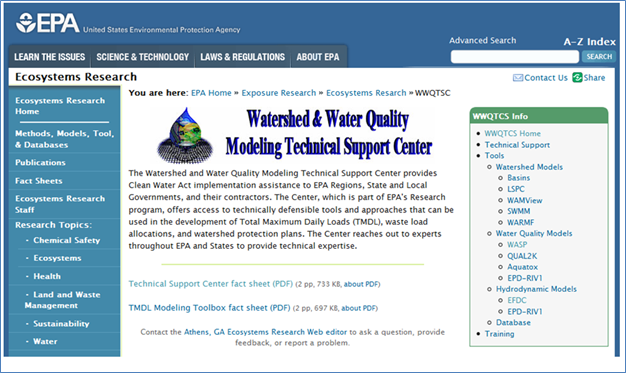
Figure 1- EPA Watershed & Water Quality Modeling Technical Support Center
The current version of the EPA supported WASP7 model (Version 7.52) can be downloaded from the URL link https://www.epa.gov/exposure-assessment-models/water-quality-analysis-simulation-program-wasp
Screenshots of the WASP7 pages from the EPA website are shown below.
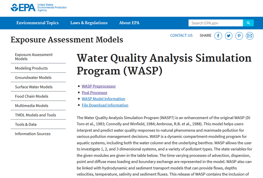
Figure 2- Water Quality Analysis Simulation Program (WASP), page 1 of 2

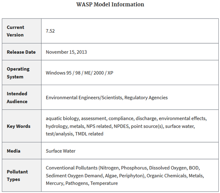
Figure 3- Water Quality Analysis Simulation Program (WASP), page 2 of 2
The current versions of the Dynamic Solutions-International EFDC model and EFDC_Explorer can be downloaded from the URL links:
http://www.efdc-explorer.com/resources/demonstration-models.html
http://www.efdc-explorer.com/downloads/efdc-explorer.html
Example Problem#1: One Dimensional (1D) Steady State River
The problem setting for the example problem is a simple steady state one-dimensional (1D) river problem. A single wastewater facility discharges CBOD and ammonia that affects the distribution of dissolved oxygen in the river. A textbook problem, taken from Thomann and Mueller (1987), is setup as an EFDC and WASP7 model to simulate flow, velocity, depth, sediment (TSS), dissolved organic carbon (CBOD), ammonia and nitrate in the river. The example problem is based on the calibration data set where the upstream river flow is 100 cfs. The wasteload allocation data set with the upstream flow of 30 cfs is not setup for the example EFDC and WASP7 problems. An analytical exact solution of the steady state 1D river model (STREAM) is setup to provide a benchmark comparison to the results shown in the textbook and the results obtained with the EFDC and WASP7 models.
The EFDC model is configured to generate a hydrodynamic (HYD) file for linkage to the WASP7 water quality model. The WASP7 water quality model is setup with the EFDC grid cell scheme and the hydrodynamic transport data from the HYD file. The textbook water quality data is assigned for the upstream and wastewater input boundary conditions as input data to the WASP7 model. The steady state results of the EFDC and STREAM models are compared graphically to the steady state results obtained with the WASP7 water quality model.
The boundary condition data required for setup of the STREAM, EFDC and WASP7 models, shown in Figure 4 through Figure 9 from the textbook, is also presented in Table 1. Kinetic data needed for the models, shown in Figure 6, is given in Table 2.
As shown in Figure 4, the spatial domain of the textbook problem covers a distance of 30 miles from the wastewater discharge at x=0 miles to the downstream boundary at x=30 miles. The EFDC domain is setup with the upstream boundary at x=50,000 meters and the downstream boundary at x=0 meters. The wastewater discharge is located 2500 meters (1.6 miles) downstream of the upstream boundary.
The EFDC 1D river problem is setup using N=100 grid cells with upstream inflow at the north boundary, lateral wastewater discharge on the west boundary and outflow at a constant elevation head from the south boundary (Figure 11). The geometry of each grid cell is DY=30.5 meters in width and DX=500 meters length for the 50,000 meter domain. An arbitrary bottom elevation of 100.0 meters was assigned for the downstream boundary cell. With a constant channel slope of 1.0e-4 m/m assigned to simulate hydrodynamic transport in the river, the bottom elevation at the upstream boundary cell is defined as 105.0 meters. Bottom elevation of the river is shown in Figure 12 and the channel slope and water depth is shown in Figure 13. The textbook problem uses empirical hydraulic relationships to define depth, width, and velocity as a function of flow in the channel. With a channel slope of 1.0e-4, a constant roughness height of 0.1 meters (Z0) was determined by “calibration” of the hydrodynamic model to best match the textbook velocity of 0.1 meter/sec. A constant downstream elevation head of 101.0 meters was assigned to control a constant depth of 1.0 meters in the channel to best match the depth of the textbook problem.
Salinity is not considered in the textbook problem. However, in order to show how salinity and water temperature are linked from the EFDC hydrodynamic model for input to the WASP7 model, salinity is activated as a state variable (Figure 15). The boundary conditions for salinity of 0.1 ppt for upstream and the wastewater discharge result in freshwater “tidal” concentrations of 0.1 ppt salinity in the 1D river with a very minor effect on the oxygen saturation concentration at T=25 C.
In the textbook problem, water temperature is assigned as 25 Deg-C. In the EFDC model, water temperature is simulated with “no atmospheric linkage” so that the EFDC simulation of water temperature is consistent with the textbook problem setting (Figure 16).
The textbook problem does not consider suspended sediment (TSS). Cohesive sediments are activated in the example problem to illustrate how to setup a sediment problem in EFDC (Figure 17,Figure 18, and Figure 19).
Water quality state variables of EFDC model used for the textbook problem are Dissolved Organic Carbon (DOC), Ammonia-N, Nitrate-N and dissolved oxygen. Organic matter in the textbook problem is represented as CBODU (Ultimate). Organic matter in EFDC is represented as the particulate (POC) and dissolved (DOC) forms of Organic Carbon (Figure 20). In the EFDC model setup, labile POC=0 , refractory POC=0 and DOC is assigned boundary concentrations equivalent to the CBODU concentrations shown in Table 1 for the upstream inflow and the wastewater discharge. The equivalent DOC concentration is computed from CBODU and the oxygen:carbon stoichiometry ratio (O2:C) of 2.67 gO2/g C as follows:
TOC=DOC = CBODU/ O2:C
Reference
Thomann, R.V. and J.A. Mueller (1987) Principles of Surface Water Quality Modeling and
Control. Harper & Row, New York, NY.
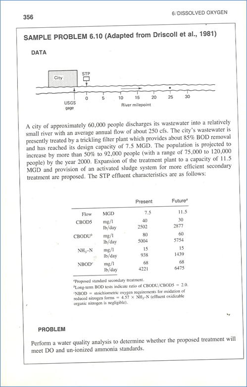
Figure 4- Thomann & Mueller (1987), Sample problem 6.10, page 1 of 6
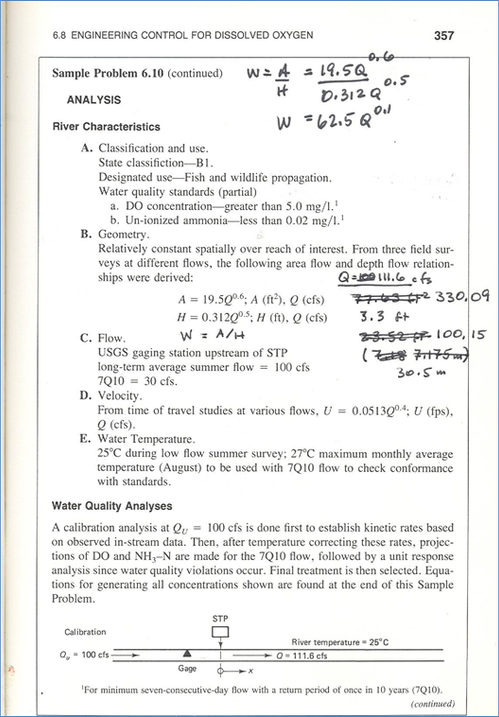
Figure 5- Thomann & Mueller (1987), Sample problem 6.10, page 2 of 6
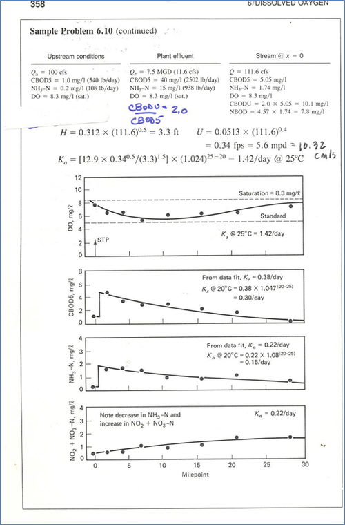
Figure 6- Thomann & Mueller (1987), Sample problem 6.10, page 3 of 6
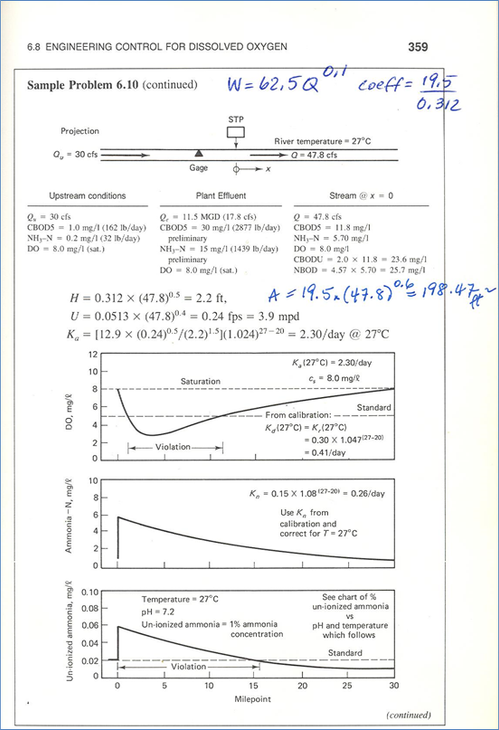
Figure 7- Thomann & Mueller (1987), Sample problem 6.10, page 4 of 6
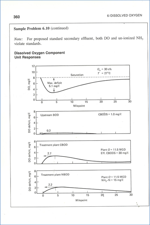
Figure 8- Thomann & Mueller (1987), Sample problem 6.10, page 5 of 6
Figure 9- Thomann & Mueller (1987), Sample problem 6.10, page 6 of 6
Table 1- Input Data for 1D River Problem
Thomann & Mueller (1987) | Sample Problem 6.10 | ||
Upstream | WWTP | ||
Flow | ft3/s | 100.0 | 11.6 |
Flow | mgd | 7.5 | |
CBOD5 | mg/L | 1.0 | 40.0 |
CBODU:CBOD5 | ratio | 2.0 | 2.0 |
CBODU | mg/L | 2.0 | 80.0 |
Oxygen | mg/L | 8.3 | 8.3 |
Oxygen Saturation | % | 100.0 | 100.0 |
Water Temperature | oC | 25.0 | 25.0 |
Ammonia-N | mg/L | 0.2 | 15.0 |
Nitrate-N | mg/L | 0.5 | 0.0 |
O2:C | ratio | 2.67 | 2.67 |
DOC=CBODU/2.67 | mg/L | 0.75 | 29.96 |
POC | mg/L | 0.0 | 0.0 |
TSS | mg/L | 2.0 | 40.0 |
Geometry/Hydraulic Data | |||
Flow (Q) | ft3/s | 111.6 | |
m3/s | 3.160 | ||
Velocity (U) | ft/s | 0.338 | U=0.0513*Q^0.4 |
m/s | 0.103 | ||
Depth (H) | ft | 3.296 | H=0.312*Q^0.5 |
m | 1.005 | ||
Area (A) | ft2 | 330.091 | A=19.5*Q^0.6 |
m2 | 30.666 | ||
Width (W) | ft | 100.149 | W=A/H |
m | 30.525 | ||
Model Domain | |||
Upstream | River Mile | -1.6 | River Meter |
WWTP | River Mile | 0.0 | River Meter |
Downstream | River Mile | 30.0 | River Meter |
Table 2- Kinetic Input Data for 1D River Problem
Kinetic Input Data | |||
Water Temperature |
| 25 | oC |
Depth |
| 3.296 | ft |
Velocity |
| 0.338 | ft/s |
Oxygen Re-aeration | O'Connor-Dobbins | 12.900 |
|
Theta | 1.024 |
| |
Ka(25) | 1.412 | /day | |
CBOD Decay | Kr(25C) | 0.380 | /day |
Theta | 1.047 |
| |
Kr(20C) | 0.302 | /day | |
Nitrification Rate | Kn(25C) | 0.220 | /day |
Theta | 1.080 |
| |
Kn(20C) | 0.150 | /day | |
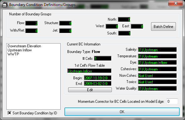
Figure 10- Boundary Conditions for 1D River.
Upstream inflow is at cell (3,102). Wastewater inflow is at cell (3,98) and the downstream elevation boundary for outflow is at cell (3,3).
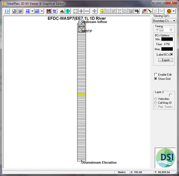
Figure 11- Boundary Condition Location Map for 1D River
Figure 12- Bottom Elevation of 1D River
Figure 13- Channel Slope and water depth of the 1D River
Figure 14- Active Modules for 1D River Problem
Figure 15- Salinity.
Initial condition set as 0.1 ppt. Boundary conditions for upstream and wastewater inflows are assigned constant 0.1 ppt.
Heat/Temperature Option for “No Atmospheric Linkage” is selected to simplify application for textbook problem. Initial conditions assigned as 25 Deg-C. Boundary conditions for upstream and wastewater inflows are assigned constant 25 Deg-C.
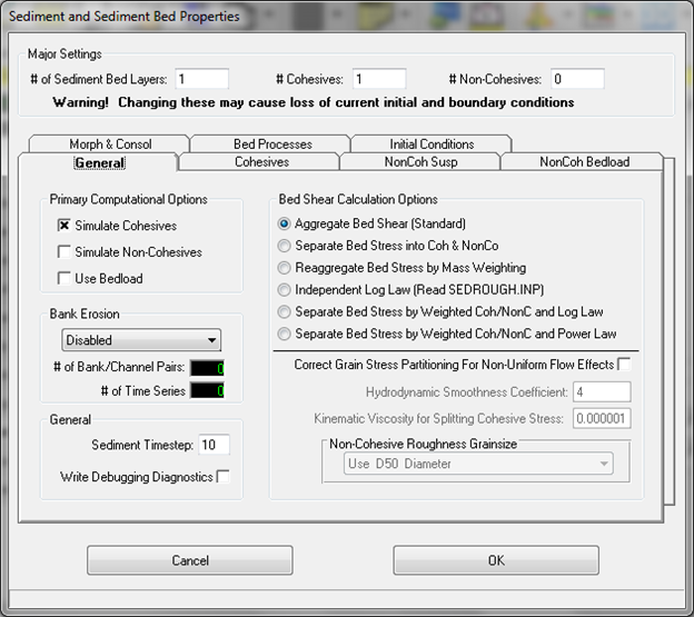
Figure 17-Cohesive Sediment.
One class of cohesive sediment is setup for example problem. One bed layer is required for sediment transport model.
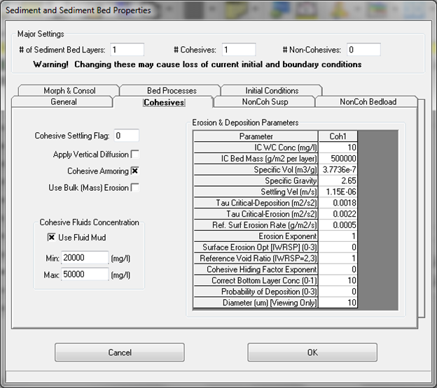
Figure 18- Cohesive Erosion and Deposition Parameters.
Settling velocity of 1.15e-6 m/s is equivalent to 0.1 m/day. Critical stresses, based on shear stress computed by hydrodynamic model, are assigned so that deposition and resuspension does not occur with shear stress from stream velocity of 0.1 m/sec. Sediment transport model is simplified with settling loss as the only process that controls the spatial distribution of cohesive sediment.
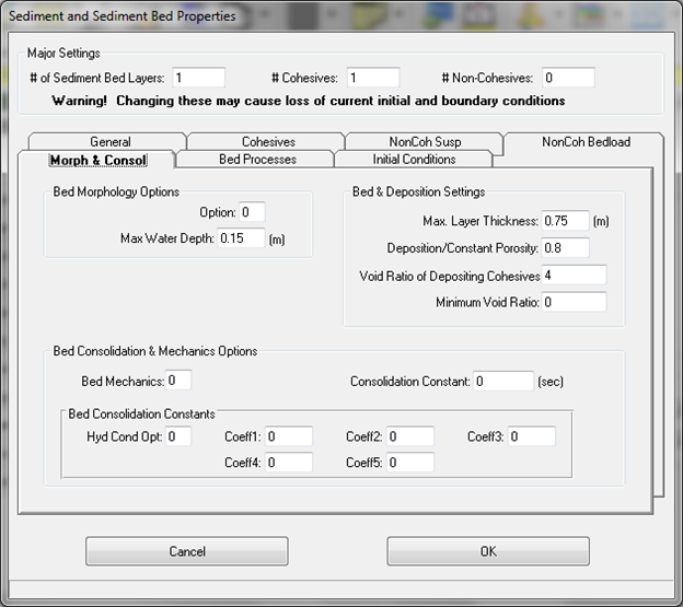
Figure 19- Bed Morphology and Consolidation.
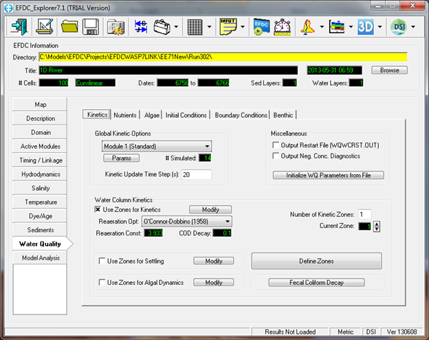
Figure 20- Water Quality. Module 1 (Standard) selected.
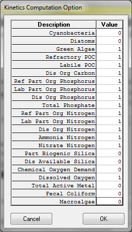
Figure 21- Active state variables for WQ module 1.
Initial conditions are assigned =0 for all state variables. Boundary conditions are assigned =0 for all state variables except for Dissolved Organic Carbon, Ammonia, Nitrate and Oxygen. Data given in Table 1 is used to assign boundary conditions for textbook problem settings for Dissolved Organic Carbon, Ammonia, Nitrate and Oxygen.
 Figure 22- Kinetic coefficients and parameters of the EFDC water quality model.
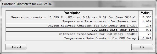
Figure 23-COD&DO Constants.
O’Connor-Dobbins coefficient and temperature dependence is assigned to match the textbook problem. The reaeration coefficient of 3.933 for O’Connor-Dobbins is for metric units of meters and m/sec for depth and velocity. The reaeration coefficient value of 12.9 shown for the textbook problem is used for units of feet and ft/sec for depth and velocity.
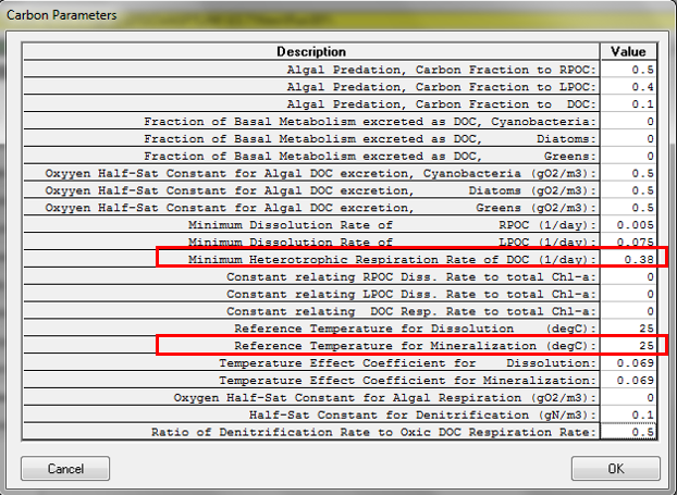
Figure 24- Carbon Parameters.
The decay rate for CBODU in the textbook problem is given as 0.38/day at T=25 Deg-C. The Carbon coefficients for minimum heterotrophic respiration rate for DOC =0.38 and the reference temperature =25 Deg-C are assigned for EFDC input to match the textbook data for decay of organic matter.
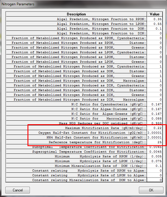
Figure 25- Nitrogen Parameters.
The nitrification rate for Ammonia in the textbook problem is given as 0.22/day at T=25 Deg-C. The Nitrogen coefficients for maximum nitrification rate =0.22 /day and the reference temperature =25 Deg-C are assigned as EFDC input to match the textbook data for nitrification. The half saturation constants for Oxygen and NH4 are assigned small values of 0.00001 mg/L so that the formulation used for nitrification in EFDC gives as close a match as possible to the textbook problem for the nitrification rate used for each grid cell of the 1D model. See Figure 26 for the nitrification equation used in EFDC.

Figure 26- Nitrification equation used in the EFDC water quality model (Tetra Tech, 2007).
Tetra Tech (2007). The Environmental Fluid Dynamics Code Theory and Computation, Volume 3: Water Quality Module. Prepared by Tetra Tech, Inc., Fairfax, VA, June.
The units in Tetra Tech (2007) for the maximum nitrification rate are incorrectly given as g N/m**3-day. The correct units for this parameter Nitm are 1/day at a water temperature of TNit as given in Ji (2008).
Ji, Zhen-Gang (2008). Hydrodynamics and Water Quality: Modeling Rivers, Lakes, and Estuaries. John Wiley & Sons, Inc., Hoboken, NJ.
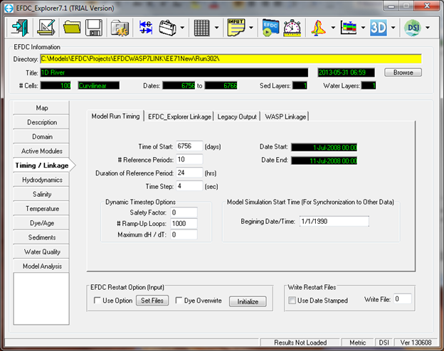
Figure 27- Timing and Linkage for 1D River Problem.
1/1/1990 is assigned as the reference base date. The simulation begins on 1 July 2008 (day=6756) and ends 10 days later. A time step of 4 seconds is used to maintain a stable solution.
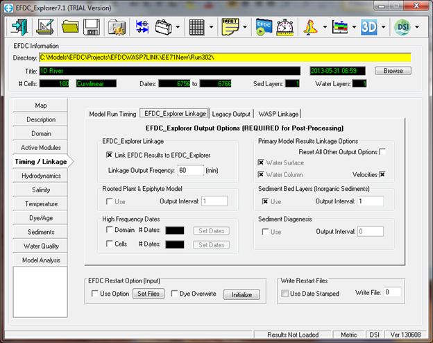
Figure 28- EFDC Explorer Linkage.
EFDC results are written to output files at 60 minute intervals.
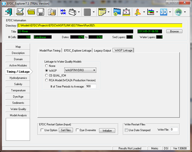
Figure 29- WASP Linkage.
WASP7HYDRO is selected from the drop down list for WASP linkage. The # Time periods to average is assigned 900 to match the 60 minute output interval assigned for EFDC Explorer linkage. With a time step of 4 sec and an EFDC output interval of 60 minutes (=3600 seconds), the EFDC model results are averaged over 900 iterations (900 =3600 sec/4 sec DT).
EFDC-WASP7 Linkage Control File EFDC.WSP
Successful generation of an EFDC hydrodynamic linkage (HYD) file requires (a) setup of an EFDC hydrodynamic model; and (b) user created input control file named EFDC.WSP. A description of the data provided in the EFDC.WSP file is presented in the EFDC Hydro user’s manual. The User manual can be downloaded from EPA website:
https://www.epa.gov/exposure-assessment-models/efdc-manuals
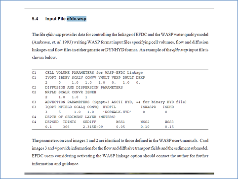
Figure 30- Input File EFDC.WSP from EFDC-HYDRO User Manual.
EFDC.WSP is an ASCII text file that can be created in any text editor. As shown in the code shown below, the filename EFDC.WSP is hardwired in the EFDC model source code that uses the control file to support generation of the EFDC HYD file for linkage to WASP7. The EFDC.WSP control file must be located in the same folder used for all the EFDC project input files.
c for jswasp=1 only first entry
OPEN(1,FILE='EFDC.WSP',STATUS='UNKNOWN')
The current version of the EFDC source code that can be obtained from Dynamic Solutions International uses a version of the EFDC.WSP control file for creation of the EFDC HYD file that is similar, but not identical, to the record structure shown in the above screenshot from the EFDC-HYDRO user manual (Figure 30).
Screenshots of the EFDC.WSP file used for the 1D River problem are shown below. The EFDC.WSP text file is included in the files provided for this sample problem.
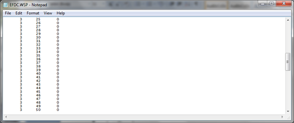
Figure 31- EFDC.WSP Control File used for 1D River problem, page 1 of 2.
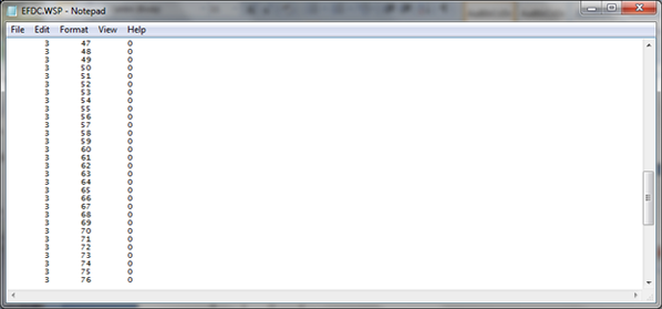
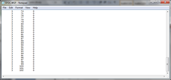
Figure 32- EFDC.WSP Control File used for 1D River problem, page 2 of 2
As can be seen in the data entered in the EFDC.WSP control file (Figure 31), most of the ”legacy” parameters shown in the EFDC-HYDRO manual are assigned dummy integer or floating point values of 999 or 999.0.
Card image C2 includes new data for ADCOEFF and ABMAX as shown in the C2 records below
C2 DIFFUSION AND DISPERSION Limiting PARAMETERS
C2 xxxxx xxxxx xxxxx xxxx ADCOEFF ABMAX
999 999.0 999.0 999 0.9 0.001
These two parameters are described in the EFDC.WSP control file as:
- ADCOEFF - coefficient that limit the max dispersion flux to a fraction of the volume divided by the time step
- ABMAX - global maximum dispersion in m2/s - this set an upper limit on the vertical dispersion
Card Image C3 is the record where the user assigns the filename for the EFDC HYD file.
C3 Hyd file name and IDAYS PARAMETERS
C3 xxxx xxxxxx xxxxxx xxxxx Hyd File Name xxxxxx xxxx IDAYS
4 999 999.0 999.0 RUN302EE71.hyd 999 999 0
Card Image C5 is where the user assigns the reference beginning date for the EFDC hydrodynamic model project. See screenshot from EFDC_Explorer for data input for the 1D river hydrodynamic project (Figure 33).
C5 Not Used
C5 iyear imon iday
1990 1 1
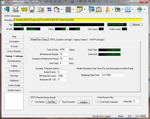
Figure 33- EFDC_Explorer Model Run Timing.
Beginning date/time for reference date for EFDC Julian day values is 1/1/1990 for the 1D river problem. EFDC Start simulation Day 6756 is 1-July-2008 00:00. Reference date is entered on Card image C5 to assign the beginning year, month, day for the WASP7 project.
After the control file input for the beginning date of the EFDC/WASP7 project the user must enter a set of data records to assign the spatial dependence of ABMAX for each horizontal grid cell (I, J) of the EFDC model domain.
C5 list of cell specific ABmax; overrides global ABMAX for cells listed; ABMAX for all cells written out to ABmax.txt file. The first few records of this part of the EFDC.WSP file are shown below.
C5 I J ABmax I J Wasp Segment Data for 1D RIVER Problem
3 3 0
3 4 0
3 5 0
The EFDC source code that reads the ABMAX data provided in the EFDC.WSP file reads in the loop from LT=2, LALT as shown below.
DO LT=2,LALT
read(1,*,err=12)i,j,abwmax
l=lij(i,j)
abwmx(l)=abwmax
write(*,*)'<EFDC.WSP7> ',i,j,abwmax
ENDDO
12 continue
The sequence of the data records in the loop LT=2, LALT reads each horizontal grid cell in the EFDC project in a sequence identical to the loop used to read EFDC input data from the DXDY.INP file as shown in the screen shot of the file for the 1D river problem (Figure 34).
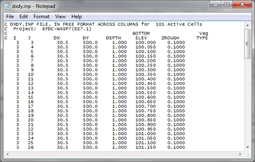
Figure 34-DXDY.INp file for 1D river problem.
The first two data columns provide the sequence of all horizontal (I, J) grid cells that are required for correct setup of the EFDC.WSP control file. The user can prepare a correctly formatted EFDC.WSP file by importing the DXDY.INP file into Excel to get the correct sequence of I and J grid cells. Insert a third column after the imported I, J records from the DXDY.INP and insert the assignment of ABMAX value (as m2/s) desired for each grid cell for the WASP7 model.
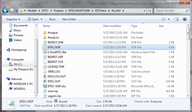
Figure 35—EFDC.WSP and other Input files for 1D river problem.
EFDC.WSP file must be located in the folder for the EFDC project input files.
Linkage of EFDC Generated HYD file and Setup of WASP7 Project
Successful generation of an EFDC hydrodynamic linkage (HYD) file requires (a) setup of a working EFDC hydrodynamic model; and (b) user created input control file EFDC.WSP as described above. The EFDC model writes the hydrodynamic (HYD) file for linkage to the WASP7 project to the EFDC project folder …………….. \#output\wasp\ (see Figure 36). The EFDC HYD hydrodynamic linkage file is used to setup a new WASP7 project as described in Ambrose and Wool (2009).
Ambrose, R.A. and T. Wool (2009) WASP7 Stream Transport- Model Theory and User’s Guide, EPA/600/R-09/100, September.
Section 4.1.4 and 4.1.5 text presented below is taken from Ambrose and Wool (2009)
4.1.4 Hydrodynamics
There are currently three surface flow options available for WASP. The first two options pertain to how WASP will calculate the exchange of mass between adjoining segments with flow in both directions across a segment interface. The three flow options available for surface water flow are:
1. Gross Flows -- WASP will calculate net transport across a segment interface that has opposing flow. WASP will net the flows and move the mass from the segment that has the higher flow leaving. If the opposed flows are equal no mass is moved.
2. Net Flows -- Pertains to mass and water being moved without regard to net flow.
3. Kinematic Wave -- For one-dimensional, branching streams or rivers, kinematic wave flow routing is a simple but realistic option to drive advective transport. The kinematic wave equation calculates flow wave propagation and resulting variations in flows, volumes, depths, and velocities throughout a stream network.
4. Hydrodynamic Linkage -- Realistic simulations of unsteady transport in rivers, reservoirs, and estuaries can be accomplished by linking WASP7 to a compatible hydrodynamic simulation. This linkage is accomplished through an external “hyd” file chosen by the user at simulation time. The hydrodynamic file contains segment volumes at the beginning of each time step, and average segment interfacial flows during each time step. WASP7 uses the interfacial flows to calculate mass transport, and the volumes to calculate constituent concentrations. Segment depths and velocities may also be contained in the hydrodynamic file for use in calculating reaeration and volatilization rates. Before using hydrodynamic linkage files with WASP, a compatible hydrodynamic model must be set up for the water body and run successfully, creating a hydrodynamic linkage file with the extension of *.hyd. This is an important step in the development of the WASP input file because the hydrodynamic linkage file contains all necessary network and flow information. When Hydrodynamic Linkage is selected in the Data Set Parameters screen, the user cannot provide any additional surface flow information. When you are ready to begin the development of a WASP input deck, simply open the hydrodynamic linkage file from within the data preprocessor. The hydrodynamic linkage dialog box allows the user to browse and select a hydrodynamic linkage file. The data preprocessor will open the hydrodynamic interface file and extract the number of segments, the starting and ending time. The data processor will also determine the set of boundary segments (segments that receive flow from outside the model network) and set the boundary concentrations to 1.0 mg/L. Once a hydrodynamic linkage file is selected in the data preprocessor, WASP has enough information to execute a simple test run with no loads or kinetics enabled. This step is recommended to test the network and transport integrity. If the simulation is run for a sufficient duration, concentrations should approach 1.0 mg/L throughout the network. If you are getting a number other than 1 mg/L, you may have to use a different time step in the hydrodynamic model. This is especially true if the concentrations are oscillating between large and small numbers, a clear indication of numerical instability. WASP has the ability to get hydrodynamic information from a host of hydrodynamic models. If a hydrodynamic model does not support the WASP linkage it is relative straightforward to create a hydrodynamic linkage file (see Appendix X for file format). The hydrodynamic models that currently support the WASP7.x file format are: EFDC (three dimensions), DYNHYD (one dimension branching), RIVMOD (one dimension no branching, CE-QUAL-RIV1 (one dimension branching), SWMM/Transport (one dimension branching, SWMM/Extran (one dimension branching)
4.1.5 Solution Technique
The user now has the ability to select the model solution technique to be used by the water quality module during the simulation. Currently there are 3 solution techniques that can be selected: 1) Euler – which is the traditional solution technique that has been in WASP since its inception, 2) COSMIC Flux Limiting – this solution technique is typically used when WASP is linked to multi-dimensional hydrodynamic models like EFDC, 3) Runge-Kutta 4 step solution technique used for diurnal simulations.
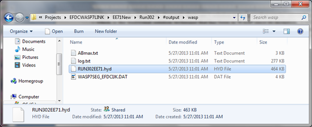
Figure 36- EFDC generated HYD file RUN302EE71.HYD for 1D river problem.
Usage of the EFDC Generated HYD File
A step-by-step sequence of screen shots is shown in Figure 37 through Figure 46 to illustrate how to link the EFDC generated HYD file to setup and save a new WASP7 project.

Figure 37- Startup screen when WASP7 is opened.
Pre-processor button is grey so data cannot be entered yet. Click on File and select the first item in drop down list to define a ‘New’ file.
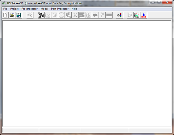
Figure 38- After clicking “New “ the pre-processor button is now ready to import the EFDC HYD file.
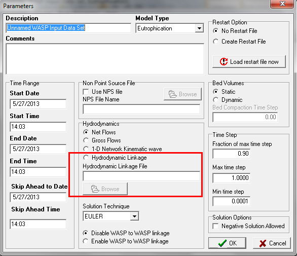
Figure 39- When you click on Pre-Processor, this screen is opened.
This is the screen where you load the EFDC HYD file. Click the button for ‘Hydrodynamic Linkage File’ and use the browser to locate the EFDC HYD file generated for the project. EFDC writes the HYD file to the EFDC project folder ………………..\#output\wasp\
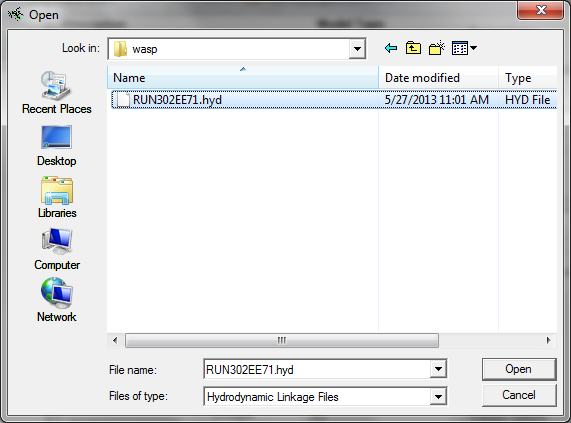
Figure 40- EFDC generated HYD file for 1D river problem.
Select and open the HYD file in the WASP7 screen. Path is shown in Figure 36 for the EFDC HYD file for the project.
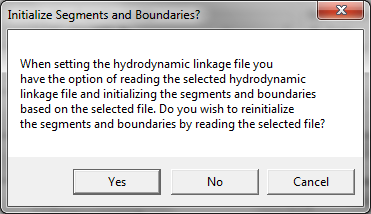
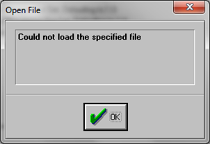
Figure 41- Message from WASP7 when HYD file is selected.
Select ‘Yes’ to setup the new WASP7 project for the 1D river problem.
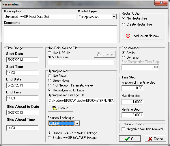
Figure 42- EFDC HYD file has been selected.
Click OK to read the HYD file.
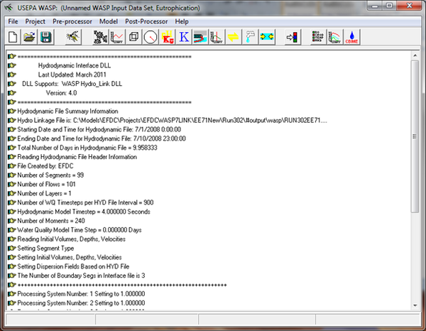
Figure 43- Data read from EFDC HYD file for the 1D river problem, page 1 of 2.
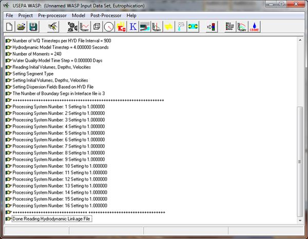
Figure 44- Data read from EFDC HYD file for the 1D river problem, page 2 of 2.
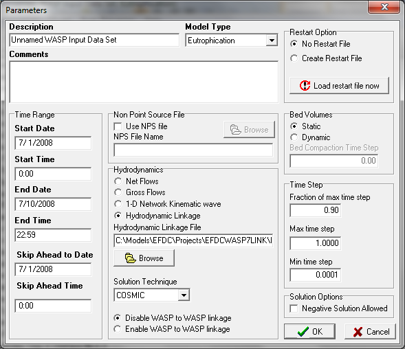
Figure 45- Pre-processor page beginning and ending date and time.
Beginning and ending date/time shown as 7/1/2008 00:00 and 7/10/2008 22:59 for the model run. Note that the solution technique has correctly been changed from EULER to COSMIC because the HYD linkage has been correctly read by WASP7. User can enter project name and description of the run/problem etc in space at top of the screen. Next step is to save the new WASP7 project file as *.WIF.
Go back to “File” button on main screen and click ‘Save As’ project file, then you use browser to save the WASP7 project file to the folder for WASP7 projects (not EFDC projects).
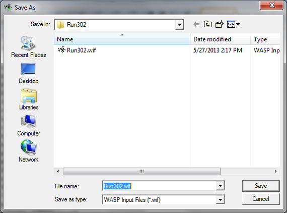

Figure 46- WASP7 project file saved in WASP7 project folder (not the EFDC project folder).
The next set of steps in setting up the WASP7 project is the input of boundary condition data for each state variable and each boundary segment. Screenshots shown in Figure 47 through Figure 56 show the assignment of default boundary condition data and testing the boundary condition settings for the 1D river problem.
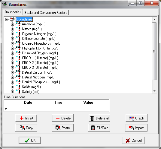
Figure 47- Pre-Processor Selection for Boundaries brings up this screen after you click on (+) sign for Boundaries.
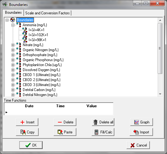
Figure 48- Click on Ammonia (+) and list of boundary segments is displayed.
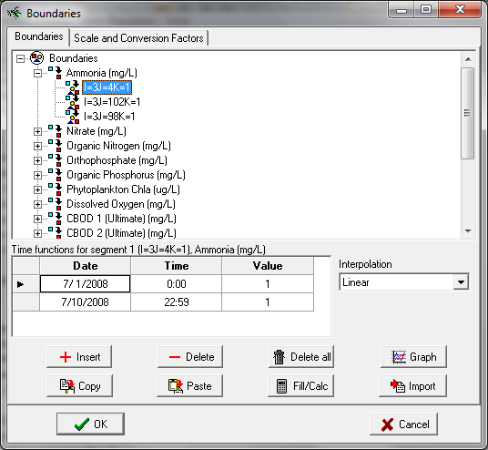
Figure 49- Default boundary settings for Ammonia.
Click on segment I=3 J=4 K=1 (which is downstream boundary segment) and the default setting of 1.0 for boundary condition data is displayed in the Time Function screen. Ammonia boundary value of 1.0 is set for begin date/time 7/1/2008 00:00 and end date/time 7/10/2008 22:59.
WASP7 assigns a default setting of 1.0 for all boundary conditions for all state variables. WASP7 boundary segments are setup with linkage data for EFDC grid cell model domain.
When setting up a new WASP7 project, EPA recommends that a model run be executed at this point to test that the data provided by EFDC hydrodynamic linkage will result in a stable WASP7 model solution.
Next step is to go to main screen and execute the WASP7 model to test the boundary settings of 1.0.
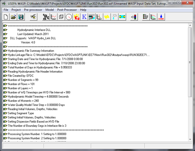
Figure 50- Click on Model and execute WASP7.
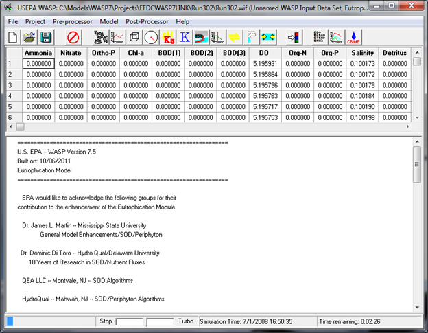
Figure 51- Screen display when WASP7 is executing.
Estimate of time remaining for WASP7 model run is shown at lower right of screen.
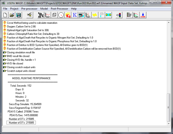
Figure 52- WASP7 run has completed successfully.
Next check the simulation results to see if model has converged to steady state solution of 1.0 mg/L at a selected grid segment. Click on Post-processor to extract time series of model results.
Message pops up; click OK and select the *.BMD file as the output results file for the WASP7 model
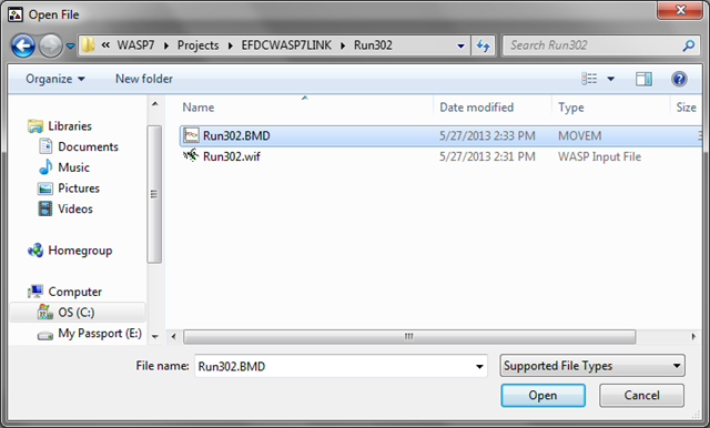
Figure 53- Select BMD file for post-processing time series results.
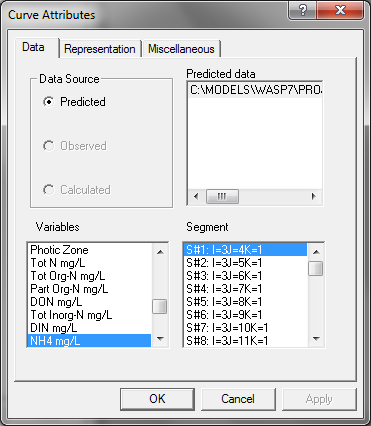
Figure 54-Select NH4 for viewing in S#1 I=3 J=4 K=1.
This is downstream boundary segment.
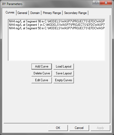
Figure 55- Select additional segments to show NH4 time series at 3 segments 98, 1 and 50.
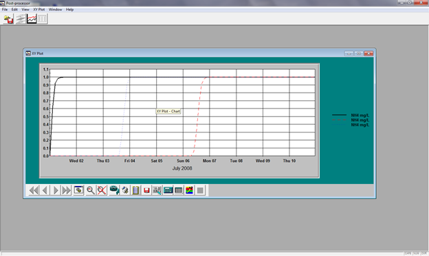
Figure 56-NH4 converges to 1.0 mg/L for 3 segments selected for display.
EFDC-WASP7 linkage is set up correctly and solution is stable.
WASP7 Boundary Condition Input for 1D River Problem
After it has been confirmed that the EFDC-WASP7 model linkage works correctly with the default boundary values of 1.0, the user must setup the actual boundary conditions and kinetic constants for each state variable for the WASP7 project. Screenshots shown in Figure 57 through Figure 61 illustrate the input of the 1D river problem boundary data to the WASP7 model.
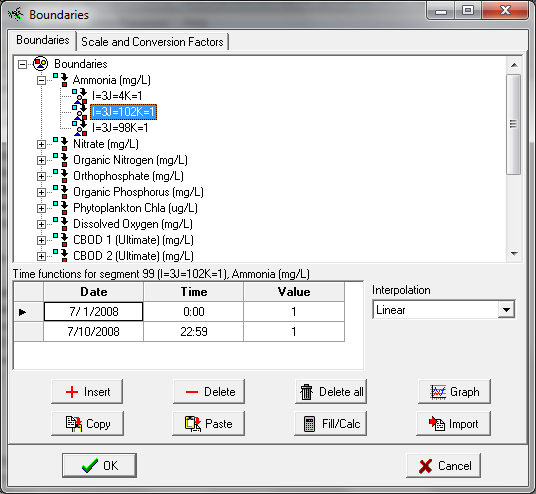
Figure 57- Boundary condition concentrations for the 1D river problem.
Boundary data for Ammonia, Nitrate, CBOD1 and Dissolved Oxygen is given in Table 1 upstream segment (I=3 J=102 K=1) and wastewater discharge segment (I=3 J=98 K=1).
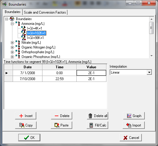
Figure 58- Upstream boundary conditions for Ammonia, NH4=0.2 mg/L.

Figure 59- Wastewater boundary conditions for Ammonia, NH4=15 mg/L.
Upstream and wastewater boundary data is assigned using the same procedure for Nitrate using boundary data from Table 1.
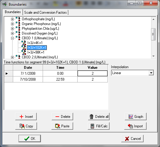
Figure 60- Upstream boundary conditions for CBOD1.
CBOD in Wasp7 is ultimate CBOD. The data given in Table 1 shows that upstream CBOD5 =1 mg/L and BOD Ultimate/5-day ratio=2 so CBOD Ultimate=2 mg/L for upstream boundary. WASP7 allows for up to 3 classes of CBOD. The 1D river problem uses only CBOD1 as the state variable for CBOD Ultimate. CBOD2 and CBOD3 are not simulated so boundary data does not have to be assigned.
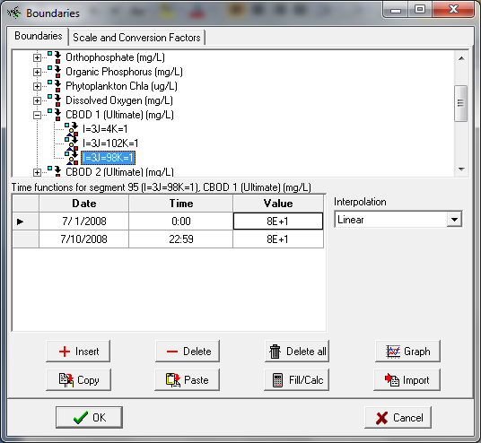
Figure 61- Wastewater boundary conditions for CBOD1.
The data given in Table 1 shows that wastewater CBOD5 =40 mg/L and BOD Ultimate/5-day ratio=2. CBOD Ultimate=80 mg/L is assigned for the wastewater boundary.
Upstream and wastewater boundary data is assigned for Dissolved Oxygen using data from Table 1. 100% oxygen saturation at Water Temperature 25 Deg-C is assigned as boundary concentration of 8.3 mg/L for upstream and wastewater discharge.
Model Parameters and Kinetic Coefficients Input for 1D River Problem
Model parameters and kinetic coefficients used for the 1D river problem are presented in Table 2. Kinetic data is input to WASP7 as ‘Constants Data’ for ammonia, nitrate, dissolved oxygen and CBOD1 as shown in the screenshots (Figure 62 to Figure 65).
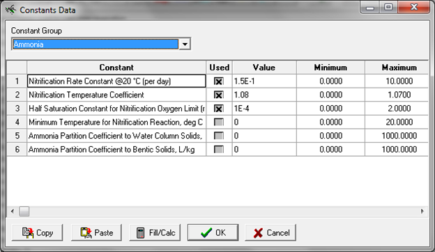
Figure 62- WASP7 Constants for Ammonia.
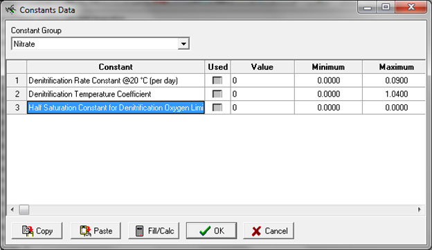
Figure 63- WASP7 Constants for Nitrate.
No nitrate constants need to be assigned for 1D rive r problem.
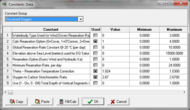
Figure 64- WASP7 Constants for Dissolved Oxygen (Reaeration Option 1=O’Connor-Dobbins).
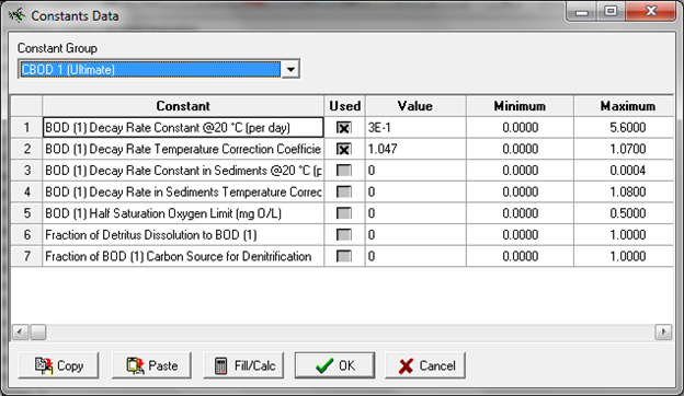
Figure 65- WASP7 Constants for CBOD1.
WASP7 Model Output and Post Processing Results
Output Control allows the user to write CSV files for selected model output variables. Data is written to CSV files as a flat data block file for all time intervals for all segments. CSV files are selected for a number of model output variables as shown in screenshots for Figure 66 to Figure 68.
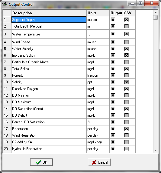
Figure 66- Output Control selection of CSV files for 1D river problem, Page 1 of 3.
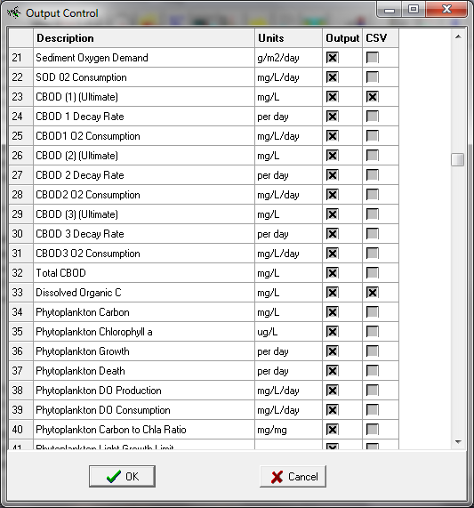
Figure 67- Output Control selection of CSV files for 1D river problem, Page 2 of 3.
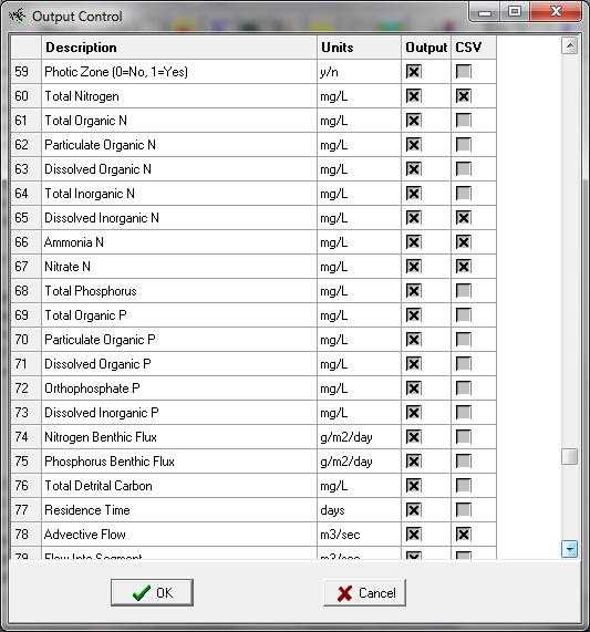
Figure 68- Output Control selection of CSV files for 1D river problem, Page 3 of 3.
Comparison of Model Results for Analytical (STREAM), EFDC and WASP7 Models
The display of steady state model results for the WASP7 model requires that a table be prepared by the user to match the WASP7 segment with a corresponding longitudinal profile x-axis coordinate for the 1D river. The upstream end of the river domain is shown in Figure 69 and the downstream end of the domain is shown in Figure 70. Model results are presented in Figure 71 through Figure 81 for depth, velocity, water temperature, salinity, CBOD5, CBODU, Total Organic Carbon (TOC), Ammonia, Nitrate, Total Nitrogen and Dissolved Oxygen.
As can be seen in the data plots, model results for both EFDC and WASP7 are in very good agreement with the analytical solution STREAM model for depth (Figure 71), velocity (Figure 72), water temperature (Figure 73), CBOD5 (Figure 75), CBODU (Figure 76), Total Organic Carbon (TOC) (Figure 77), ammonia (Figure 78), nitrate (Figure 79), Total Nitrogen (Figure 80), and dissolved oxygen (Figure 81). The good comparison of both EFDC and WASP7 with the analytical STREAM model benchmark solution confirms that the code used in EFDC and WASP7 is correct for ammonia, nitrate and dissolved oxygen state variables.
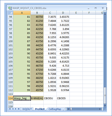 Figure 69- Data table matching Wasp7 segments with 1D river distance, upstream.
WASP Segment 99 is the upstream segment of model domain. Segment 99 extends from 50,000 to 49,500 meters. Model results plotted at midpoint of segment at 49,750 meters.
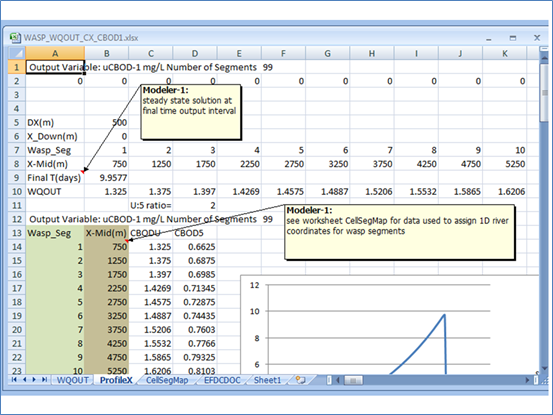
Figure 70- Data table matching Wasp7 segments with 1D river distance, downstream.
WASP Segment 1 is downstream segment of model domain. Segment 1 extends from 1000 to 500 meters. Model results plotted at midpoint of segment 1 at 750 meters. EFDC grid cell (3,3) extends from 500 to 0 meters in EFDC domain. WASP7 linkage drops downstream grid cell and assigns this cell as WASP7 segment ‘0’ boundary segment. Longitudinal profile of WASP7 steady state model results are extracted for final time interval of 9.9577 days from CSV output file data block of time and segment.
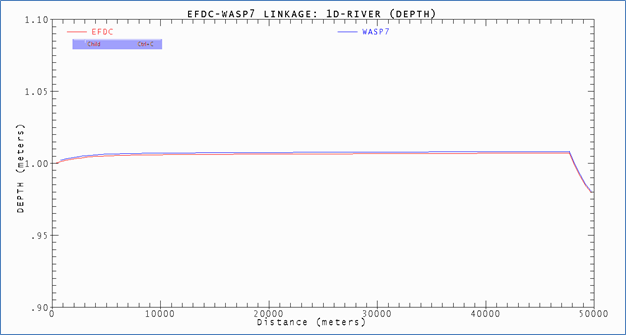
Figure 71- EFDC and WASP7 results for Stream Depth.
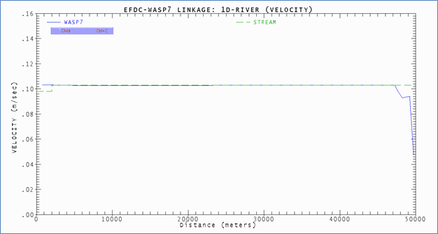
Figure 72- WASP7 and STREAM Model results for River Velocity.
Longitudinal profile of EFDC velocity is not extracted from EFDC_Explorer.
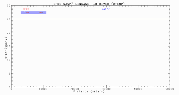
Figure 73- EFDC and WASP7 Model results for Water Temperature.
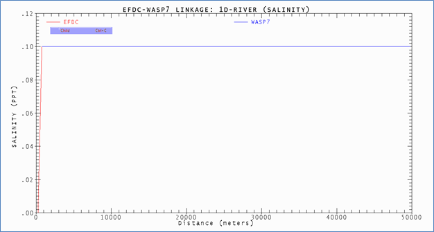
Figure 74- EFDC and WASP7 Model results for Salinity.
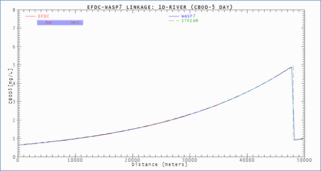
Figure 75- EFDC, STREAM and WASP7 Model results for CBOD5.
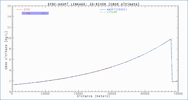
Figure 76- EFDC, STREAM and WASP7 Model results for CBOD Ultimate.
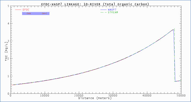
Figure 77- EFDC, STREAM and WASP7 Model results for TOC.
Note that POC=0 and TOC=DOC
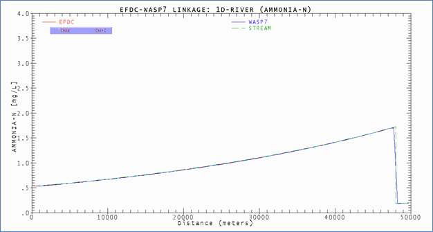
Figure 78- EFDC, STREAM and WASP7 Model results for Ammonia-N.
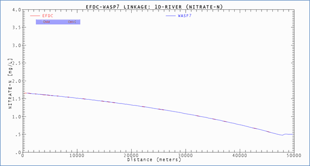
Figure 79- EFDC and WASP7 Model results for Nitrate-N.
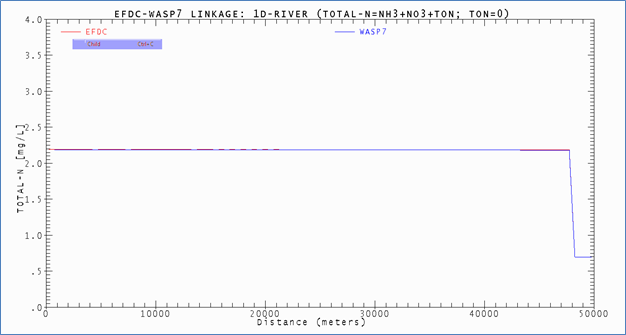
Figure 80-EFDC and WASP7 Model results for Total Nitrogen.
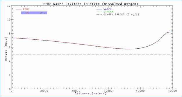
Figure 81-EFDC, STREAM and WASP7 Model results for Dissolved Oxygen.