...
This may be laid over the labels file by loading as a data posting file Figure 28(Figure 30). The measured stations and labels are shown in Figure 31.
| Anchor | ||||
|---|---|---|---|---|
|
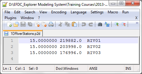
Figure 29 1DRiverStations p2d file.
Anchor Figure 30 Figure 30
...
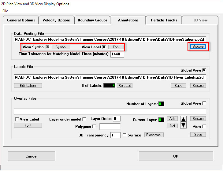
Figure 30 Loading data posting file.
...
6. Repeat this process for the WWTP series in Figure 35.
7. Repeat this process for the East Branch series, setting a flow of 0.01 (there is no flow here but we set a small flow for the dye release) shown in Figure 36.
Anchor Figure 33 Figure 33

Figure 33 Boundary condition settings: flow data series.
Anchor Figure 34 Figure 34
...

Figure 34 Boundary Condition: US flow.
Anchor Figure 35 Figure 35
...
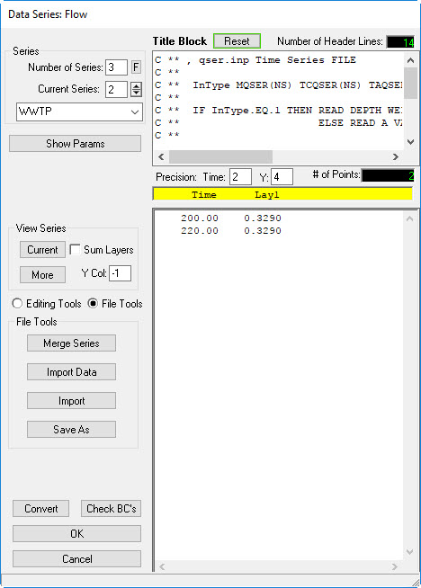
Figure 35 Boundary Condition: WWTP flow.
Anchor Figure 36 Figure 36

Figure 36 Boundary Condition: East Branch flow.
8. Return for the Main Form shown in Figure 32 and select the E button for Dye
9. Repeat the above process for dye concentrations for the Upstream (series 1) as shown in Figure 3637
10. Create Series 2 for dye concentration for “East Branch” with the same values as for “Upstream”, ie 0.2. as shown in Figure 38.
11. Create the Series 3 for “WWTP” boundaries as shown in Figure 3739.
Anchor Figure 3637 Figure 3637
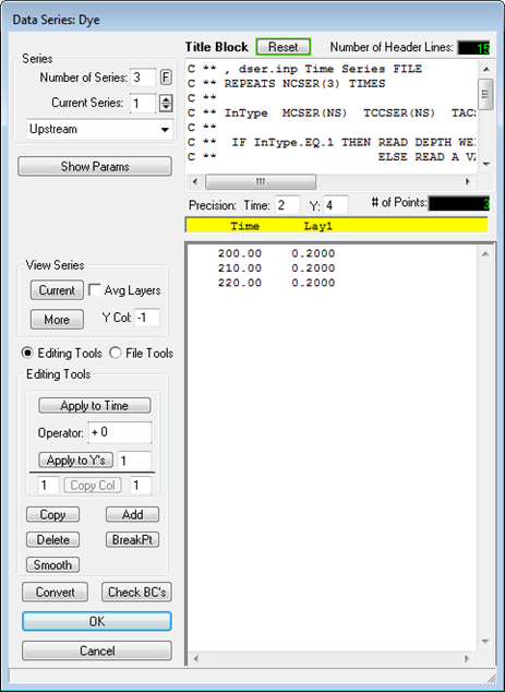
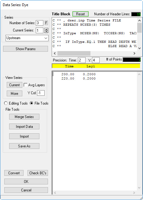 Figure 36 37 Boundary Condition: upstream dye concentration.
Anchor Figure 3738 Figure 3738
...

Figure 37 38 Boundary Condition: WWTP East Branch dye concentration.
...
Anchor
Figure 39 Figure 39
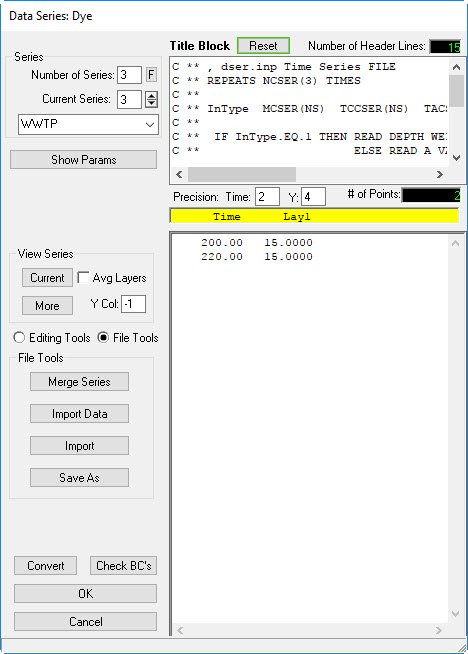
Figure 39 Boundary Condition: WWTP dye concentration.
12. Return to the Main Form and from the Active Modules tab select the Activate Dye check box to switch on dye as shown in Figure 3840.
Anchor Figure 3840 Figure 3840
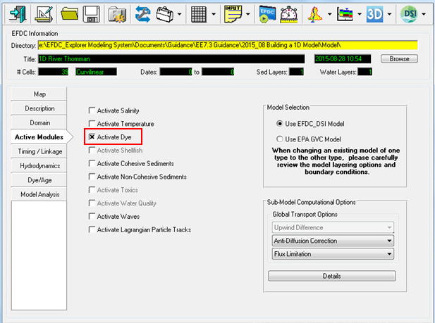
Figure 38 40 Main Form – Active Modules Tab: activate dye.
...
16. Name the BC with ID “Upstream” and select BC type = 1 for a flow boundary as shown in in Figure 3941.
Anchor Figure 3941 Figure 3941
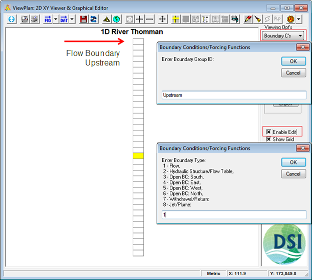
Figure 39 41 ViewPlan – Boundary Conditions: setting forcing functions.
...
The Modify/Edit BC Properties will now be displayed as Figure 42. This form is used to link the flow table to the BC.
...
19. Click E to check which series have been defined if necessary.
Anchor Figure 4042 Figure 4042

Figure 40 ViewPlan – boundary42 Modify/Edit Flow BC Properties: Upstream.
20. Click OK to return to the ViewPlan form.
...
24. Set the Flow table to “East Branch” and dye concentration series to East Branch. Click OK
Anchor Figure 4143 Figure 4143 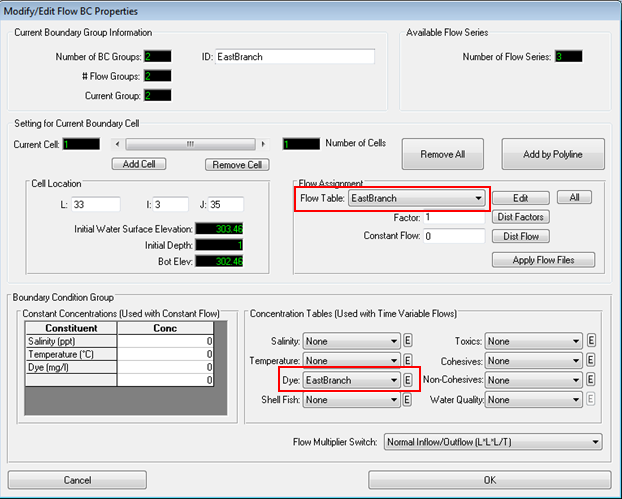
Figure 41 43 Modify/Set BC Properties: east branchEast Branch.
| Info |
|---|
Important note: A Flow Table time series must always be linked with Concentration Table (Time Variable)” flow. Conversely, a Constant concentration must always be linked to a Constant Flow. If a constant flow is selected then EE will automatically use a constant concentration, even when a flow table has been assigned. |
...
28. Set the Flow table to “WWTP” and dye concentration series to WWTP (Figure 4244), click OK
Anchor Figure 4244 Figure 4244
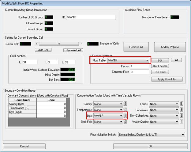
Figure 42 44 Modify/Set BC Properties: WWTP.
...
31. Select an Open BC: South option , = 3 as shown in Figure 4345. Click OK
Anchor Figure 4345 Figure 4345
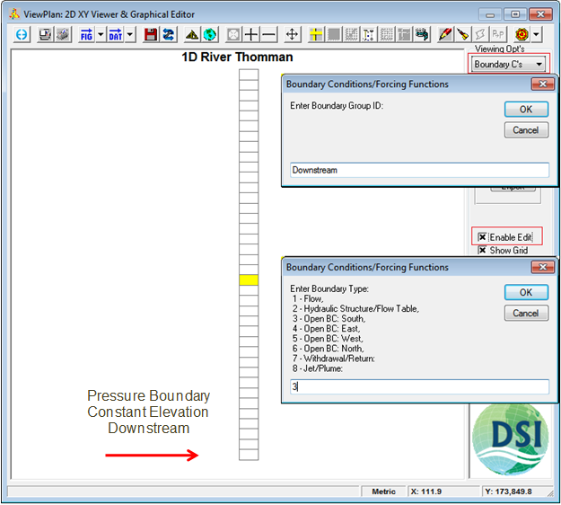
Figure 43 45 ViewPlan – Boundary Conditions: DS BC.
...
32. To set the Open Boundary, click the E (edit” button for the pressure boundary under Boundary Condition Group | Head Table or Periodic Function frame ) as shown in Figure 4446.
Anchor Figure 4446 Figure 4446

Figure 44 46 Modify/Set BC Properties: open boundary form.
...
35. Enter a constant elevation pressure of 301.000 for the time series as shown in Figure 4547 and click OK.
Anchor Figure 4547 Figure 4547
 Figure 45 47 Boundary Condition: WWTP dye concentrationDownstream water surface elevation.
36. Returning to the Modify Edit BC form,
...
38. Click Set All. Click OK.
Anchor Figure 4648 Figure 4648
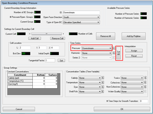
Figure 46 48 Modify/Set BC Properties: downstream open boundary.
...
All boundary conditions have now been set as shown in Figure 4749.
Anchor Figure 4749 Figure 4749
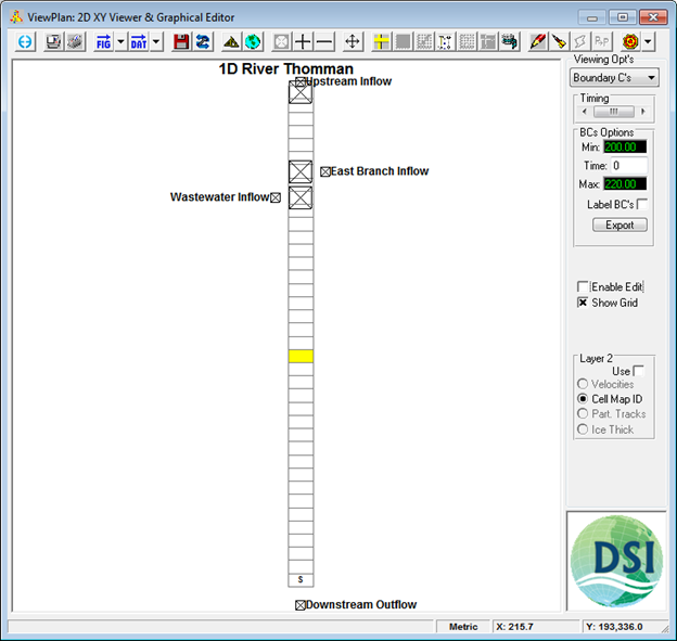
Figure 47 49 ViewPlan – BCs.
39. From the ViewPlan form, select Fixed Parameters from Viewing Options, Roughness to view the cell bottom roughness settings as shown in Figure 48. These have already been set to the default from the efdc.inp file.
...
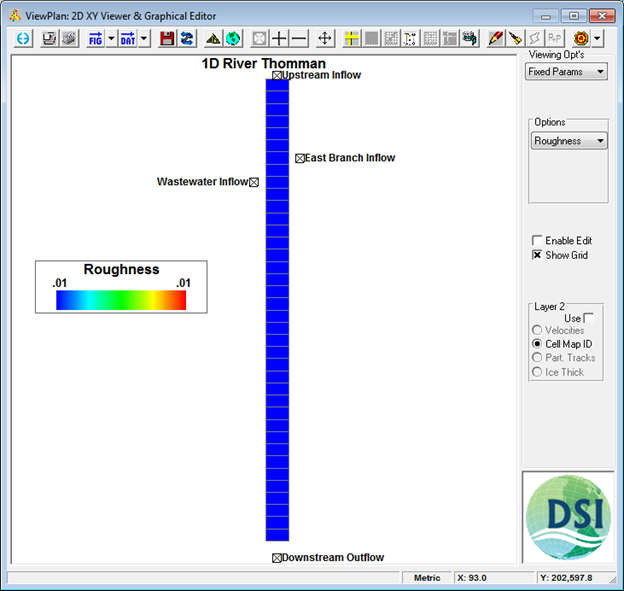
Figure 48 ViewPlan – Fixed Parameters: roughness.
5 Running the Model
...
5 Running the Model
We want to set the model to run from day 200 for 20 periods of 24 hours at a time step of 120 seconds as shown in Figure 4950.
- Save the model as shown in Section 3.2.4
- Select the Timing/Linkage tab and Model Run Timing
- Set the Model start time to 200;
- Set # of Reference Periods to 20;
- Set Duration of reference periods to 24;
- Set Time step to 120.
Anchor Figure 4950 Figure 4950
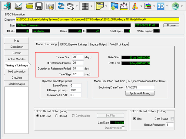
Figure 49 50 Main Form – Time / Linkage: model run timing.
...
Navigate to the EFDC_Explorer Linkage tab and set the Linkage Output Frequency to 15 minutes as shown in Figure 5051.
7. Click the Run EFDC button on the Main Form also as shown in Figure 5051.
Anchor Figure 5051 Figure 5051
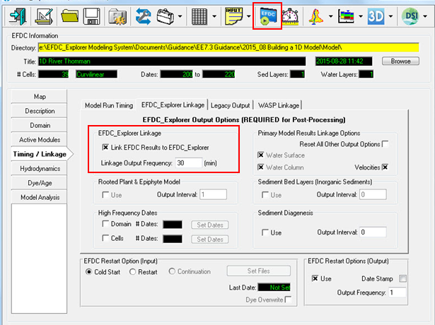

Figure 50 51 Main Form – Time / Linkage: EFDC_Explorer linkage.
...
8. Check the run options and then click the Run EFDC button as shown in Figure 52.
Anchor Figure 5152 Figure 5152
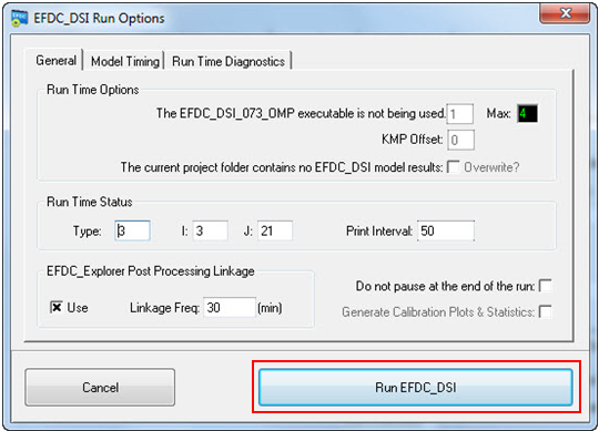
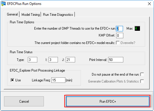
Figure 51 52 Run options.
Note that if your model doesn’t run then check that you have correctly linked EE to the EFDCPlus model on the Main Form, “Settings” button and browse to the EFDCPlus model provided. The default location is : C:\Program Files (x86)\DSI\EFDC_Explorer8EEMS8.13
6 Model Post Processing
- When the model has finished running. view the model results in the 2D ViewPlan
- Select View Options” Water by Layer and Dye from the options
- Scroll through the model run with the timing bar or using short-key Ctrl+G then enter the date (i.e 203) then click OK button
- Click the Time Series button at the top of the form (Figure 5253),
- Click on cell 3,32 and select Yes
Anchor Figure 5253 Figure 5253
...
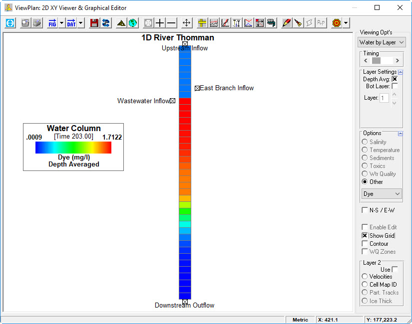
Figure 52 53 ViewPlan – Water by Layer: dye.
A time series of the dye at that cell will be displayed as shown in Figure 5354.
Anchor Figure 5354 Figure 5354
...
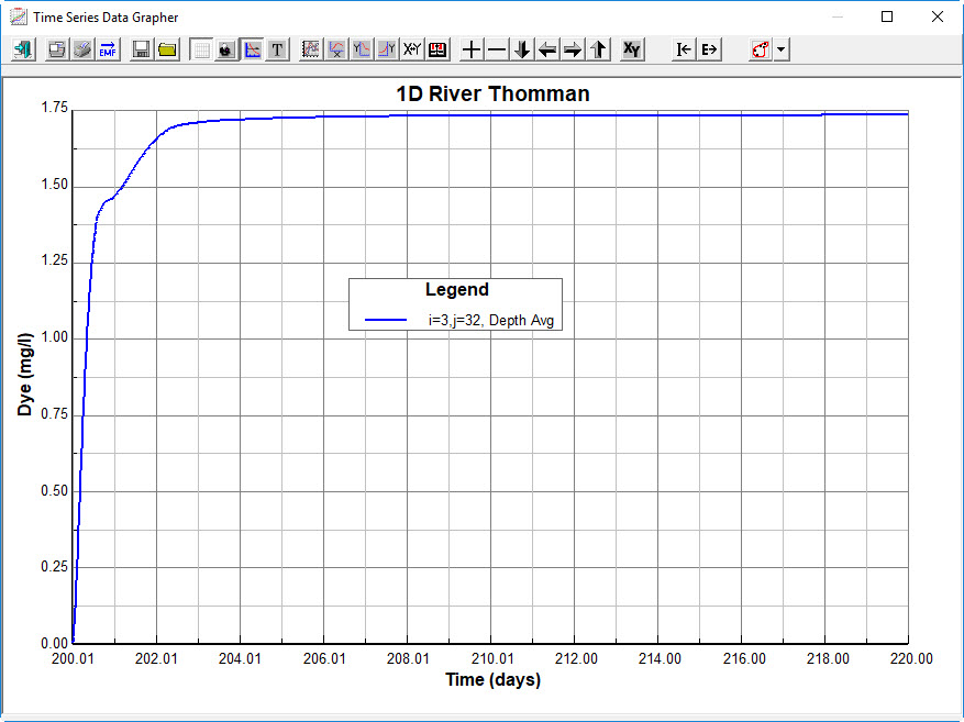
Figure 53 54 Time series data grapher: dye.
...
7 Model Calibration Tools
...
A profile plot may be set up using the Longitudinal Profile button in Figure 54 55
- Click the Longitudinal Profile button and set I=3.
- Set Line 1 to 1 to display dye as shown in Figure 5455
Anchor Figure 5455 Figure 5455
...
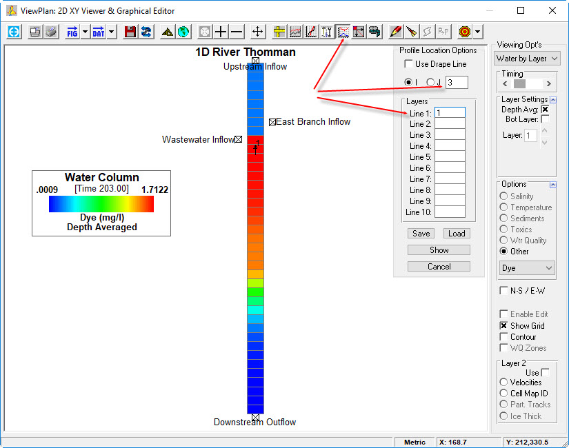
Figure 54 55 Time series data grapher.
...
4. Load the comparison file with the Import button shown in Figure 5556.
Anchor Figure 5556 Figure 5556 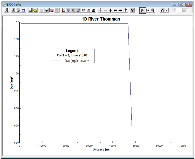
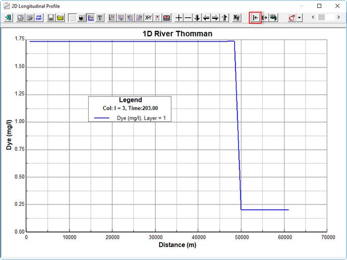
Figure 55 56 Time series data.
In order to compare to measured data we will create a file of the measured values at RIV01, RIV02 and RIV03 at time = 218 these are shown in Figure 5657.
Anchor Figure 5657 Figure 5657

Figure 56 57 Dye concentration at Time = 218.
...
5. Navigate to the .dat file containing the data from the 6. If asked if the X values are dates select “No”file containing the data as shown in Figure 58.
Anchor Figure 58 Figure 58
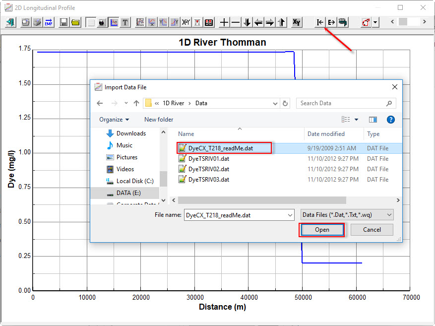
Figure 58 Loading measured data file (1).
6. If asked if the X values are dates select “No” as shown in Figure 59.
Anchor Figure 59 Figure 59

Figure 59 Loading measured data file (2).
7. Select value = 2 for the series to import the value into (modeled dye is series 1) as shown in Figure 60.
Anchor Figure 60 Figure 60

Figure 60 Enter value for timeseries data imported.
8. RMC on the legend to set the series line options for the data to dots using line plotting options as shown in Figure 5761.
9. Scroll through the timing bar or use CTRL-G to go to t=218 for comparison as shown in Figure 5862.
Anchor Figure 5761 Figure 5761

Figure 57 61 Line plotting options.
Anchor Figure 5862 Figure 5862
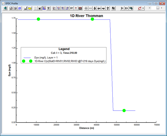
Figure 58 62 Dye concentration at Time = 218.
...
To compare with the theoretical results it is necessary to reset the dye as a non-conservative substance as shown below.
Anchor Figure 5963 Figure 5963
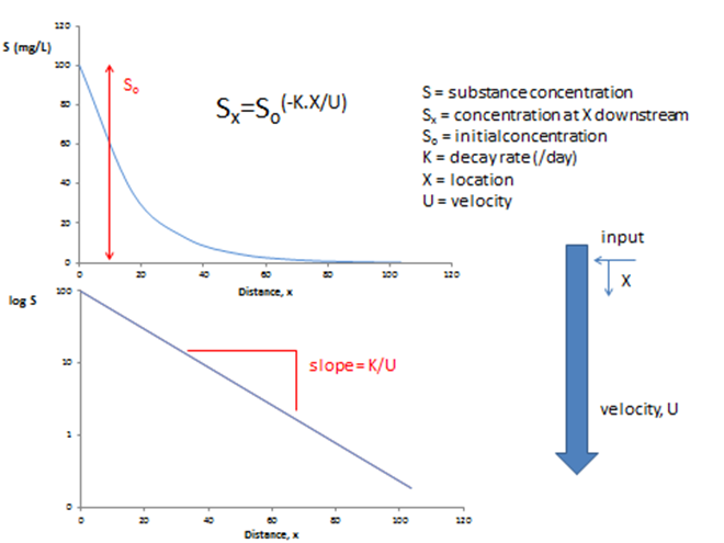
Figure 59 63 Decay of Non-conservative substances in Cartesian coordinates and Logarithmic form.
...
The resulting longitudinal profile will be like that as shown in Figure 6165.
Anchor Figure 6064 Figure 6064

Figure 60 64 Main Form – Dye: dye decay rate.
Anchor Figure 6165 Figure 6165

Figure 61 65 ViewPlan- Longitudinal Profile: K=0.15 Non-conservative dye.
...
7.3 Calibrating the Non-conservative Substance
Use the data from from Figure 6266 (provided in the file “River1D-ExactSolution.dat”) as calibration data for this project
- As described in Section 7.1 above, load the calibration data with the “I” (Import) button from the from shown in Figure 6156.
- Select No for the question are the X values dates.
- Select “2” for the value for analytical solution.
- Use CTRL G to go to time = 218
Anchor Figure 6266 Figure 6266
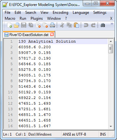
Figure 62 66 Calibration Data.
Anchor Figure 6367 Figure 6367

Figure 63 67 Dye Tracer: comparison of EFDC & analytical solution.
...
We will now compare measured data at the three station, RIV01, RIV02 and RIV03 described earlier (Figure 31). Data for these stations is as shown below in in Figure 6468 and contained in the files: DyeTSRIV01.dat, DyeTSRIV02.dat, DyeTSRIV03.dat.
5. Return to Main Form | Model Analysis | Model Calibration | Time Series Comparisons tool as shown in Figure 6569
6. Click Define/Edit
Anchor Figure 64 Figure 64
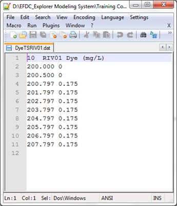
Figure 64 68 RIV01 calibration data.
Anchor Figure 6569 Figure 6569

Figure 65 69 Main Form – Model Analysis: model calibration.
...
7. Set the Number of time series to 3 as shown in Figure 6670
8. Define the X, Y value for the calibration station for each of the three stations.
...
15. Click OK
Anchor Figure 6670 Figure 6670
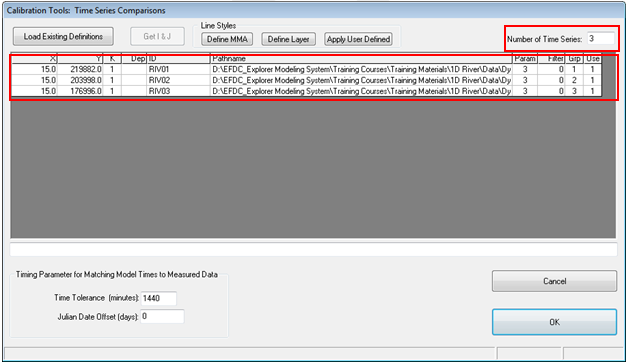
Figure 66 70 Calibration Tools – time series comparisons.
...
16. Click OK for Calibration Plot Generation Options without selecting the checkboxes to display the graph in Figure 6771.
We now want to set the data display so that is similar to that shown in Figure 6771.
17. RMC the legend
18. Select the data series and adjust the settings as shown in Figure 68
Anchor Figure 6771 Figure 6771
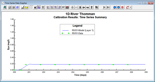
Figure 67 71 Calibration – time series comparisons: RIV01.
...
19. Click Save to save the plot settings shown in Figure 6872
Anchor Figure 6872 Figure 6872

Figure 68 72 Calibration – time series comparisons: line options and controls.
...
21. Load the previously saved Line Options and Controls settings with Load button to apply to the next plot so that it appears as shown in Figure 6973.
22. Apply the above step for RIV03 as shown in Figure 7074.
Anchor Figure 6973 Figure 6973

Figure 69 73 Calibration – time series comparisons: RIV02.
Anchor Figure 7074 Figure 7074

Figure 70 74 Calibration – time series comparisons: RIV03.
...