This tutorial document is based on a steady state problem from Thomann & Mueller (1987) “Principles of Surface Water Quality Modeling and Control” Sample Problem 6.10 (which was itself adapted from Driscoll et al., 1981).

The purpose is to provide new users of EE with a step by step tutorial to setup a simple hydrodynamic and water quality model that they can create themselves from scratch. At the same time, it provides the more advanced modeler the ability to make a comparison between analytical solution and the EFDC results.

1. Tasks to be performed

This document will take the user through the following steps:

• building a grid
• setting hydraulic parameters
• setting initial conditions
• setting boundary conditions
• setting a conservative and non-conservative dye tracer
• creating data files for calibration data
• configuring calibration plots

2. Description of the Problem

2.1 Background

The problem is taken from Thomann and Mueller (1987, p.356). A city of approximately 60,000 people discharges its wastewater into a relatively small river with an average annual flow of about 250 cfs. The city’s wastewater is presently treated by a trickling filter plant which provides about 85% BOD removal and has reached its design capacity of 7.5MGD. The population is expected to increase by 50% to 92,000 people by the year 2000. Expansion of the treatment plan to capacity of 11.5 MGD and provision of an activated sludge system for more efficient secondary treatment are proposed.

A calibration analysis at Qu = 100 cfs is done first to establish kinetic rated based on observed in stream data.

2.2 Basic Data and Data Processing

2.2.1 Data Requirements

• Upstream and tributary boundary inflows of water and pollutants
• Initial conditions of water depth and pollutants in time and space
• Physical transport of water (velocity, travel time)
• Waterbody geometry (length, depth, area, volume)
• Pollutant fate reactions and interactions
• Sources/loading rates of flow & pollutants

2.2.2 River Characteristics

Geometry

Relatively constant spatially over reach of interest. From three field surveys of different flows, the following area flow and depth flow relationships were derived:

• A = 19.5Q^0.6 ; A (ft²), Q (cfs)
• H= 0.312Q^0.5; H (ft), Q (cfs)
• W = A/H

Flow

• USGS gaging station upstream of WWTP
• Long term average summer flow = 100 cfs
• 7Q10 = 30 cfs (for min 7-consecutive day flow with return period of once in 10 years)

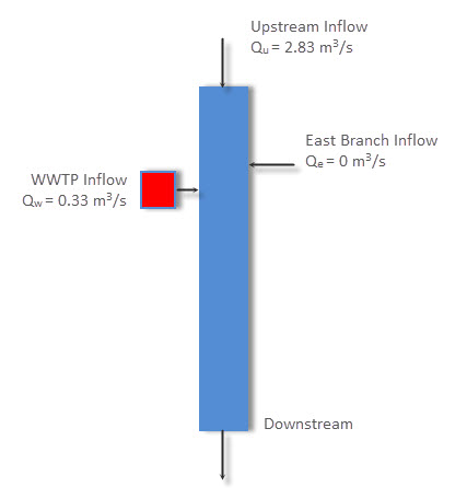
Figure 1  1-D River schematic.

Velocity

From time of travel studies at various flows, U = 0.0513Q^0.4; U (fps), Q (cfs)

Water Temperature

25 ^oC during low flow summer survey, 27 ^oC maximum monthly average temperature (August) to be used with 7Q10 to check conformance with standards.

H = 0.312 x (111.5)^0.5  = 3.3 ft

U = 0.0513 x (111.6)^0.4 = 0.34 fps = 5.6 mpd = 10.32 cm/s

K_a = [12.9 x 0.34^0.5 / (3.3)^1.5] x (1.024)^25-20 = 1.42 /day @25 ^oC

2.3 Model Input Data

Upstream boundary

• Located at x = 227,030 m
• Upstream inflow Q_u= 2.83 cms  (100 cfs)
• Upstream bottom elevation = 303 m

East Branch inflow (note that this inflow can be ignored and is not in the original example)

• Located at x = 216,705.5 m
• Q_e=0

Waste Water Treatment Plant

• Located at x = 213,528.7 m
• Q_w = 0.33 cms (7.5 mgd, 11.6 cfs)

Downstream boundary

• Located at x = 165,083 m
• Downstream bottom elevation = 300 m
• Flow below WWTP =  3.16 cms  (100 + 11.6 =111.6 cfs)

Area-Depth-Velocity Relationships as f (flow, cfs)

• Area = 19.5*Q^0.6 =330.1 ft² = 30.67 m²
• Depth = 0.312*Q^0.5 = 3.3 ft = 1.006 m
• Velocity = 0.0513*Q^0.4 =0.34 ft/s = 0.1036 m/s
• Width = Area/Depth = 100.15 ft ~ 30.0 m
• Grid cell length DY=1588.4 m
• Total length of 1D river = 61,947.0 m
• Number of Grid Cells = 39
• Constant head for downstream elevation control = 301 m.

User experience and trial and error method to determine appropriate slope and bottom roughness

• Bottom roughness:  Z₀ = 0.06 m
• Channel slope = - 0.5 e-4 m/m 
• Cell depths computed by EFDC model from channel slope and upstream & downstream bottom elevations

3. Generating a New Model

3.1 Generate a New Model

3.1.1 Generating a Grid

In this step, we will generate a simple model grid to present the 1D river in our problem.

   1. Open EFDC_Explorer.

   2. From the empty main form shown in Figure 2, select the Generate New Model button

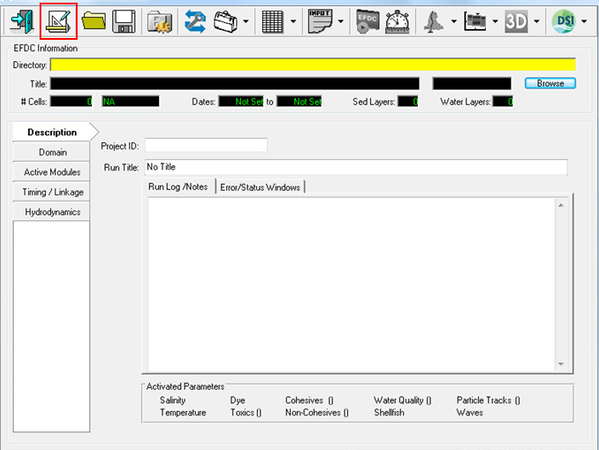
Figure 2  EFDC_Explorer main form.

The form shown in Figure 3 should now be displayed.

  Figure 3  Generate EFDC model.

   3. Select Cartesian Grid Type | Uniform Grid for this case.

   4. Leave Rotation Angle = 0 as we won’t rotate the grid

We will now enter values for Lower Left and Upper Right of model domain. These These values correspond to the US and DS boundary conditions outlined in Model Input Data above

   5. Set Lower Left:                        Easting = 0, Northing = 165,083

   6. Set Upper Right:                     Easting = 30, Northing = 227,030

   7. Grid Cell Length, Delta  = 30 and 1588.4 for X and Y respectively

   8. Press Update to update the number of X and Y cells.

   9. Select Flat Bottom for Elevation Options (we normally set a flat bottom and add bathymetry later)  

   10. Enter a bottom elevation = -1

   11. Leave # Corners = 0

 When all the necessary information has been provided the Generate button will be available as shown in Figure 4. If the form is missing some information the Generate button is greyed out.

12. Press Generate and a message box will appear as shown in Figure 5.

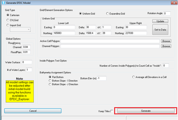
Figure 4  Generate EFDC model – with data.

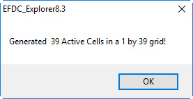
Figure 5  Generate grid message box.

Viewing and Checking the Grid

Once the model grid is created, we can display and check the grid.

In the Main Form, the model domain is now displayed on the Map tab (Figure 6)

   1. Click the the View 2D Plan button on the main menu to see the model in plan view.

Figure 6  Main form – map tab.

   2. Select Cell Map from View Options in the right hand column to view the model cell map (Figure 7)

   3. Select Label Cells from Cell Map Options

The I and J cell map is displayed. The filled cell is the centroid of the model domain.

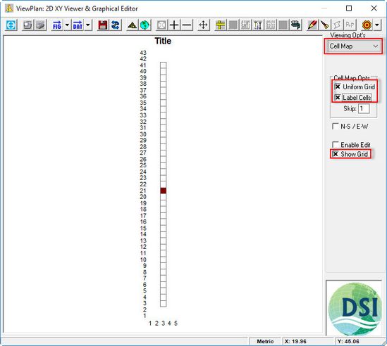
Figure 7  ViewPlan - Cell Map with I & J labels.

    4. Select Bottom Elevation from the Viewing Options drop down menu as shown in Figure 8.

This now displays the bottom elevation of the model domain. As the model is very long and narrow, it is hard to see clearly. To increase the width of the model, the user must use horizontal exaggeration.

Figure 8  2D ViewPlan – bottom elevation.

   5. Click the Display Options button ( the 8th button on the top menu from the left of the 2D Viewplan form) or RMC on the legend in ViewPlan to bring up the ViewPlan Display Options as shown in Figure 9.

   6. Set the Easting value to 100 in the E/N Scales Modifiers frame. This will stretch the model by a factor of 100 in the Y direction and is easier to view.

   7. Change the Plot Title to “1D River- Thomann”

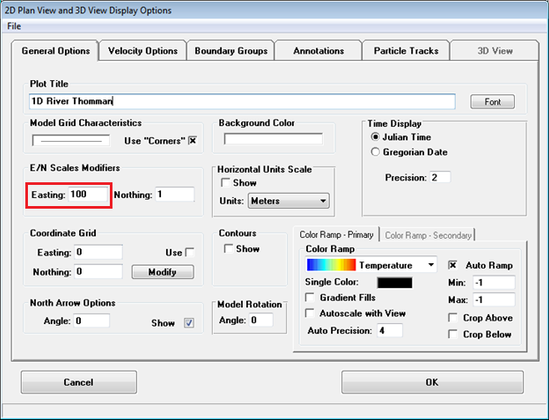
Figure 9  2D ViewPlan – Display Options: general options.

Now we want to better understand the Cell Indices of our model.

   8. Select Cell Indices in the Viewing Options drop down and select Show I & J’s from the Options as shown in Figure 10.

   9. Click on any of the cells in the model domain to display an information box (yellow) that describes the cell L number, I and J number, the X, Y coordinates, bottom elevation and depth.

Figure 10  2D ViewPlan – cell indices.

3.1.2 Checking the Longitudinal Profile

Another view that is helpful for the user to determine the vertical profile of the model is with the Vertical Profile option shown in Figure 11

   1. Select the ViewProfile button

The Extraction Options form shown in Figure 12 should now be in view. Using this form the user may select a profile along a pre-defined polyline or along an I or J entered by the user.

   2. In this case select I=3.

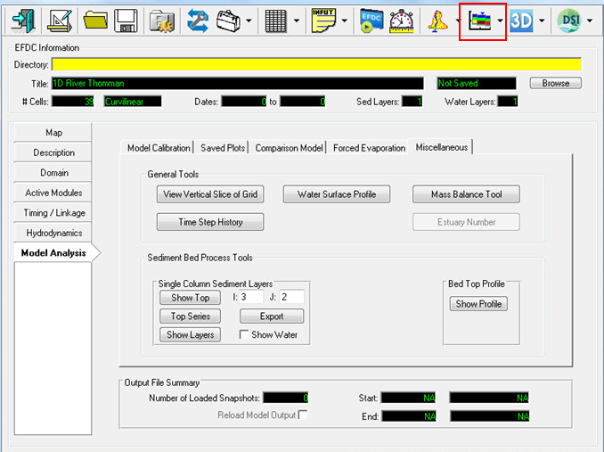
Figure 11  Main Form – Vertical Profile button.

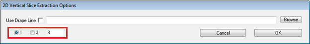
Figure 12  2D ViewProfile.

   3. The vertical profile is shown in Figure 13. The horizontal distance is shown on the X-axis and the elevation on the Y-axis. The user may adjust titles, units and formatting by RMC on either axis.

   4. RMC on the legend provides allows you to set the parameter to be viewed.

Figure 13  Vertical Profile – Density.

Another option to display the longitudinal profiles:

   1. Return to the 2D ViewPlan form.

   2. Select the Longitudinal Profile button as shown in Figure 14, and enter an I value of 3.

   3. Hovering the mouse over the Layers options shows that various lines may be displayed.

   4. In this case we will select the WSEL and the Bottom Layer, -1 and -3 respectively.

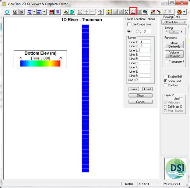
Figure 14  2D ViewPlan – Longitudinal Profile selection.

   5. If necessary, adjust the plot so that both lines are displayed on the left hand axis by RMC the legend and selecting Water Surface in the Line Options and Controls and then in General Options, Y-axis frame switch to the left hand Y axis as shown in Figure 16.

   6. Adjust the thickness of the lines until they display satisfactorily with the Line Formatting option.

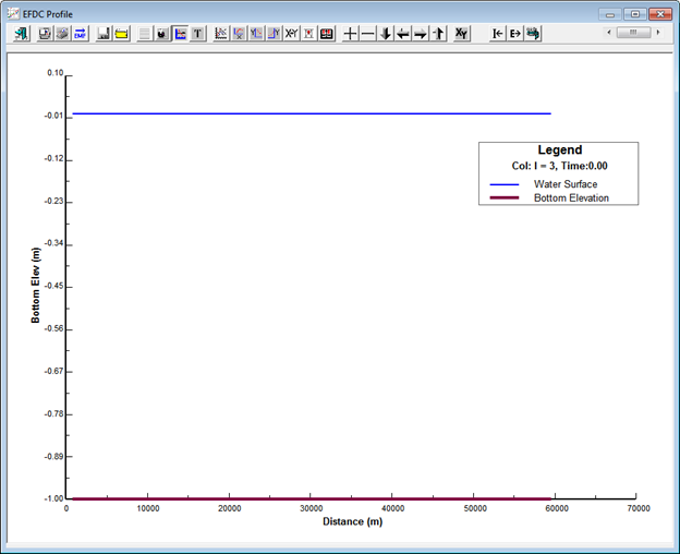
Figure 15  2D ViewPlan – Longitudinal Profile.

Figure 16  2D ViewPlan – Longitudinal Profile: line options.

3.2 Assigning Initial Conditions

In this step, we will setup the initial conditions for bottom, water surface elevations and bottom roughness.

3.2.1 Assigning Bathymetry

   1. Return to the Main Form and select the Domain tab and Initial Conditions and Bottom Roughness sub-tab to set the bathymetry and water surface elevations as shown in Figure 17.

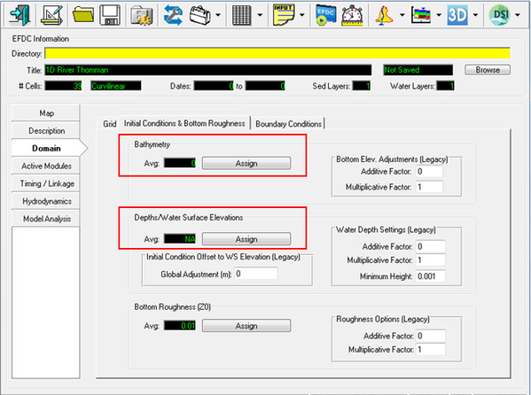
Figure 17  Main Form – Domain Tab: IC and bottom roughness.

   2. Select the Assign button for bathymetry to displays the form shown in Figure 18.

   3. Select Bottom Slope – J direction from the Adjustment Options and set elevation = 300 and the slope to - 0.00005. Note that this is a negative slope to assign from the DS to US end of the model, starting at 300 m at the DS end. 

   4. Select Apply and Done to apply these changes. EE will tell you that this has been applied to 39 cells which is all the cells in the domain.

Once the model bathymetry is assigned, we can check the data using the viewing options (2D plan view or longitudinal profiles) following the steps described in Sections 3.1.2 and 3.1.3.

Figure 18  Assigning IC for bottom elevation.

3.2.2 Assigning Water Surface Elevation

   1. Similarly, select the Assign button for Water Surface Elevation to display the form shown in Figure 19.

   2. Set the IC to Use Constant and set the constant = 1.

   3. We want to set the depths, so set the check box Assign Depths instead of WSEL.

   4. Click Apply and Done

Figure 19  Assigning IC for WSEL.

   5. To check the data, return to the 2D ViewProfile and repeat the Longitudinal Profile selection described in Section 3.1.2  to view the changes made to the vertical profile. This displays the plot shown in Figure 20.

Figure 20  Longitudinal Profile.

3.2.3 Assigning Bottom Roughness

   1. Similarly, select the Assign button for Bottom Roughness (Z0) to display the form shown in Figure 21

   2. Set the IC to Use Constant and set the constant = 0.06.

   3. Click Apply and Done

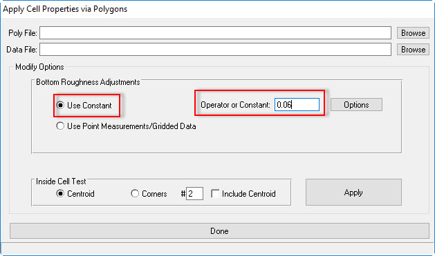
Figure 21  Assigning IC for Bottom Roughness.

3.2.4 Naming the Model

The user should enter the name of the project in the Description tab | Project ID and Run Title. These will become the default names in the ViewPlan and Time Series titles.

3.2.5 Saving the Model

1. Click on the Save button as shown in Figure 22 to save the model.
2. Use the form shown in Figure 22 to navigate to the directory that you want to save the model.
3. Create a new directory with the Create New button and name the directory.
4. Click OK to save.

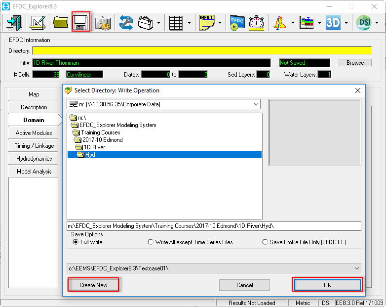
Figure 22  Main Form – save button.

3.2.5 Placing Labels in the ViewPlan

We now want to create labels for this model.

1. Open a text editor and create a simple text file with three columns, space delimited.  X, Y and Label are the three columns.

X and Y correspond to the locations that we want our boundary conditions as shown in Figure 23.

Figure 23  Creating a labels file.

   2. Save the file with the suffix .dat or p2d (note that p2d is a non-proprietary format commonly used by DSI).

   3. Proceed to the ViewPlan 2D form

   4. RMC on the legend or select the Display Options button and select the Annotations tab ( See Figure 24)

   5. From the Labels file form browse to the labels file just created and load it.

   6. Select Global View check box to view the labels.

When displayed the labels are as shown in Figure 25 and have not yet been correctly aligned and symbols have not yet been selected.

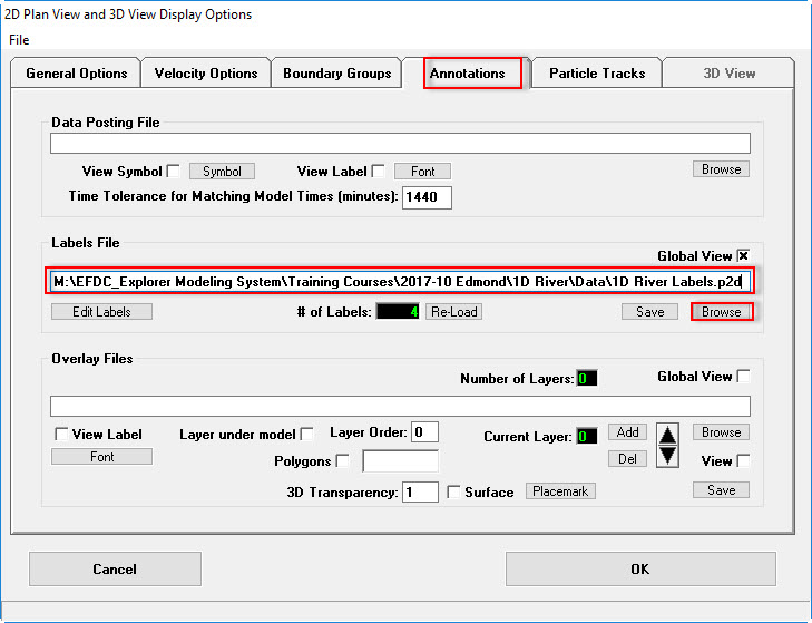
Figure 24  ViewPlan – Display Options: annotations.

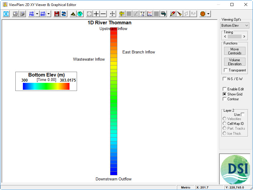
Figure 25  ViewPlan: labels.

   7. Select the Edit Labels button form the Annotation tab to correctly align the labels and set the symbols as shown in Figure 26.

Figure 26  ViewPlan – Display Options: Edit Labels.

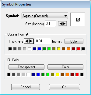
Figure 27  ViewPlan: symbol properties.

   8. Update the symbols and labels as desired such as shown in Figure 28.

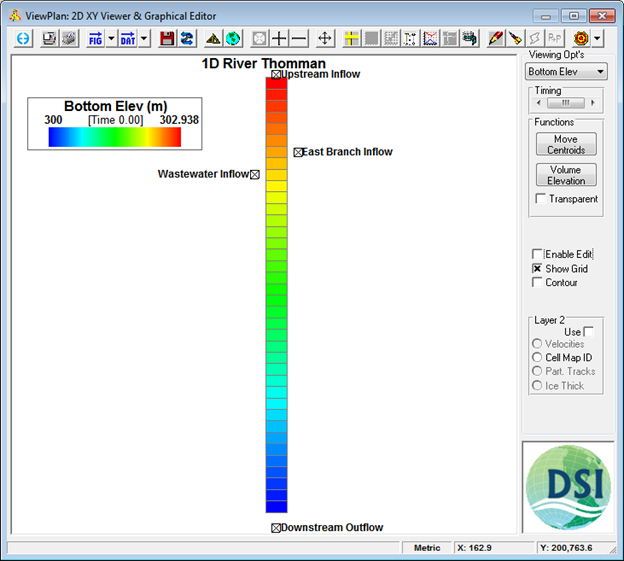
Figure 28  ViewPlan.

   9. Select Save

Once the labels are saved from the form in Figure 24, EE will create a labels file that will retain all the settings for label fonts, locations and symbols. In this case the file is called 1DRiverLabels.lbf

It is assumed for the purposes of this tutorial that three data recording stations are providing measured data. The user should create a file to record the locations of data recording stations called 1DRiverStations.p2d: (Figure 29)

This may be laid over the labels file by loading as a data posting file (Figure 30). The measured stations and labels are shown in Figure 31.

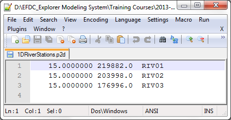
Figure 29  1DRiverStations p2d file.

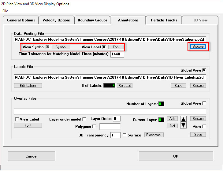
Figure 30  Loading data posting file.

Figure 31  Overlay of data posting file on labels.

4  Boundary Conditions

The boundary conditions for this model have been taken from the Thomman text book example and are summarized in the table below. In this case dye is used as proxy for the contaminant transport.

To enter these BCs into the model we will first create the time series and then set the BC locations and link them to the time series.

   1. Proceed to the Domain Tab | Boundary Conditions subtab shown in Figure 32

From this form we can create the Flow boundary time series and the Dye boundary time series

   2. Select the I for Edit button on Flow for the Number of Input Tables and Series. This will display the form shown in Figure 33.

Figure 32  Main Form – boundary condition settings.

   3. Set the number of flow series to 3 (since Downstream will be set as a WSEL or pressure boundary)

   4. Use the arrow buttons below to go to series 1 and enter the values shown in Figure 34

   5. Set the title to “Upstream” and type or copy and paste into the the form for the time and flow data. 200 represents the start time of the data series in Julian time. At least two times must be entered for each series.

   6. Repeat this process for the WWTP series in Figure 35.

   7. Repeat this process for the East Branch series, setting a flow of 0.01 (there is no flow here but we set a small flow for the dye release) shown in Figure 36.

Figure 33  Boundary condition settings: flow data series.

Figure 34  Boundary Condition: US flow.

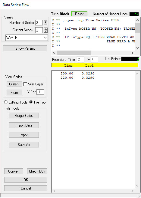
Figure 35  Boundary Condition: WWTP flow.

Figure 36  Boundary Condition: East Branch flow.

   8. Return for the Main Form shown in Figure 32 and select the E button for Dye

   9. Repeat the above process for dye concentrations for the Upstream (series 1) as shown in Figure 37

   10. Create Series 2 for dye concentration for “East Branch” with the same values as for “Upstream”, ie 0.2. as shown in Figure 38.

   11. Create the Series 3 for “WWTP” boundaries as shown in Figure 39.

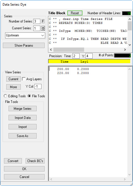Figure 37  Boundary Condition: upstream dye concentration.

Figure 38  Boundary Condition: East Branch dye concentration.

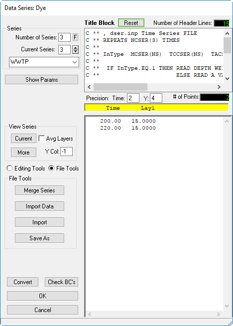
Figure 39  Boundary Condition: WWTP dye concentration.

   12. Return to the Main Form and from the Active Modules tab select the Activate Dye check box to switch on dye as shown in Figure 40.

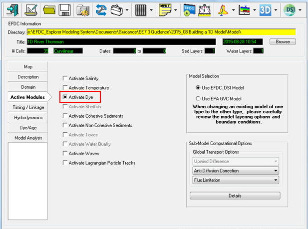
Figure 40  Main Form – Active Modules Tab: activate dye.

   13. To link the time series with the BC locations, proceed to the ViewPlan 2D form and select Boundary Conditions from the Viewing Options drop down.

   14. Select Enable Edit from the right hand column.

   15. RMC on the cell most upstream cell and select New to create a new boundary condition.

   16. Name the BC with ID “Upstream” and select BC type = 1 for a flow boundary as shown in Figure 41.

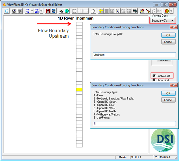
 Figure 41  ViewPlan – Boundary Conditions: setting forcing functions.

The Modify/Edit BC Properties will now be displayed as Figure 42. This form is used to link the flow table to the BC.

   17. Use the drop down table under the Boundary Condition Group | Flow Definition (Cell by Cell) | Flow Table to select the “Upstream” BC.

   18. Set the Concentration tables | Dye to Upstream. This links the Upstream flow to the Upstream dye concentration (series 1) previously defined.

   19. Click E to check which series have been defined if necessary.

Figure 42  Modify/Edit Flow BC Properties: Upstream.

   20. Click OK to return to the ViewPlan form.

   21. RMC on the cell for “East Branch” that is cell I=3, J=35.

   22. Set the Boundary group ID to “East Branch,” Click OK.

   23. Enter 1 to set flow type to Flow. Click OK

   24. Set the Flow table to “East Branch” and dye concentration series to East Branch. Click OK

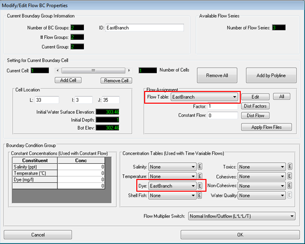
Figure 43  Modify/Set BC Properties: East Branch.

In the ViewPlan form we will now set the WWTP BC.

   25. RMC on the cell for “WWTP” that is cell I=3, J=33.

   26. Set the Boundary group ID to “WWTP,” Click OK.

   27. To set flow type to flow, enter 1 and click OK

   28. Set the Flow table to “WWTP” and dye concentration series to WWTP (Figure 44), click OK

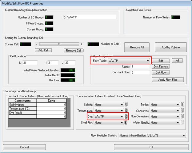
Figure 44  Modify/Set BC Properties: WWTP.

Now we will set the Downstream BC. This will use a fixed WSEL to set the pressure boundary (clamped boundary). Therefore, we set a constant head at the downstream boundary.

   29. In the ViewPlan form, RMC on the bottom most cell (I=3, J=3)

   30. Name the Boundary group “Downstream”. Click OK

   31. Select an Open BC: South option = 3 as shown in Figure 45. Click OK

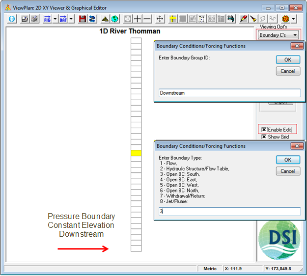
Figure 45  ViewPlan – Boundary Conditions: DS BC.

  32. To set the Open Boundary, click the E (edit” button for the pressure boundary) as shown in Figure 46.

Figure 46  Modify/Set BC Properties: open boundary form.

   33. Set Number of series to 1 and select Current series 1.

   34. Give the Title “Downstream” to this series. Select the Single option.

   35. Enter a constant elevation pressure of 301.000 for the time series as shown in Figure 47 and click OK.

  Figure 47  Boundary Condition: Downstream water surface elevation.

   36. Returning to the Modify Edit BC form,

   37. Select the new “Downstream” series from the drop down menu

   38. Click Set All. Click OK.

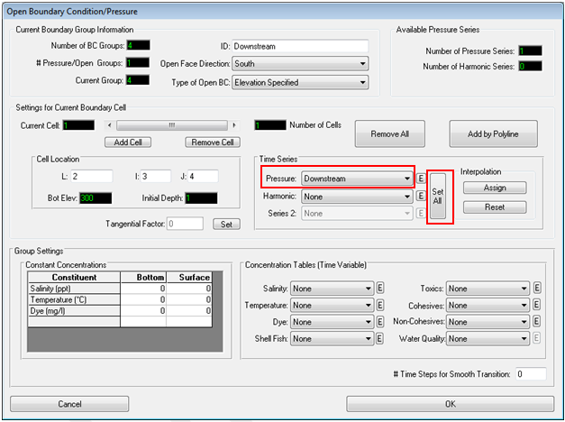
Figure 48  Modify/Set BC Properties: downstream open boundary.

All boundary conditions have now been set as shown in Figure 49.

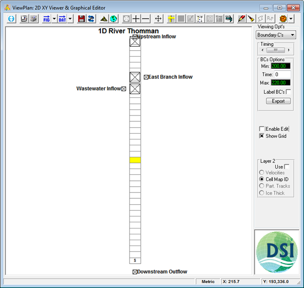
Figure 49  ViewPlan – BCs.

5  Running the Model

We want to set the model to run from day 200 for 20 periods of 24 hours at a time step of 120 seconds as shown in Figure 50.

1. Save the model as shown in Section 3.2.4
2. Select the Timing/Linkage tab and Model Run Timing
3. Set the Model start time to 200;
4. Set # of Reference Periods to 20;
5. Set Duration of reference periods to 24;
6. Set Time step to 120.

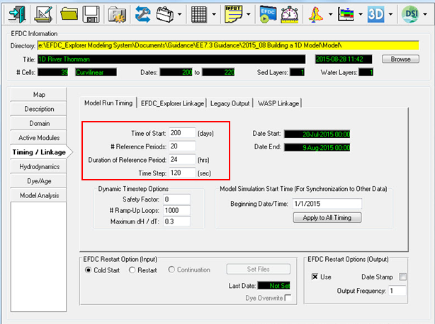
Figure 50  Main Form – Time / Linkage: model run timing.

Navigate to the EFDC_Explorer Linkage tab and set the Linkage Output Frequency to 15 minutes as shown in Figure 51.

   7. Click the Run EFDC button on the Main Form as shown in Figure 51.

Figure 51  Main Form – Time / Linkage: EFDC_Explorer linkage.

   8. Check the run options and then click the Run EFDC button as shown in Figure 52.

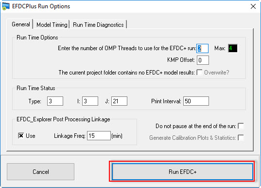
Figure 52  Run options.

Note that if your model doesn’t run then check that you have correctly linked EE to the EFDCPlus model on the Main Form, “Settings” button and browse to the EFDCPlus model provided. The default location is : C:\Program Files (x86)\DSI\EEMS8.3

6  Model Post Processing

1. When the model has finished running. view the model results in the 2D ViewPlan
2. Select View Options” Water by Layer and Dye from the options
3. Scroll through the model run with the timing bar or using short-key Ctrl+G then enter the date (i.e 203) then click OK button
4. Click the Time Series button at the top of the form (Figure 53)
5. Click on cell 3,32 and select Yes

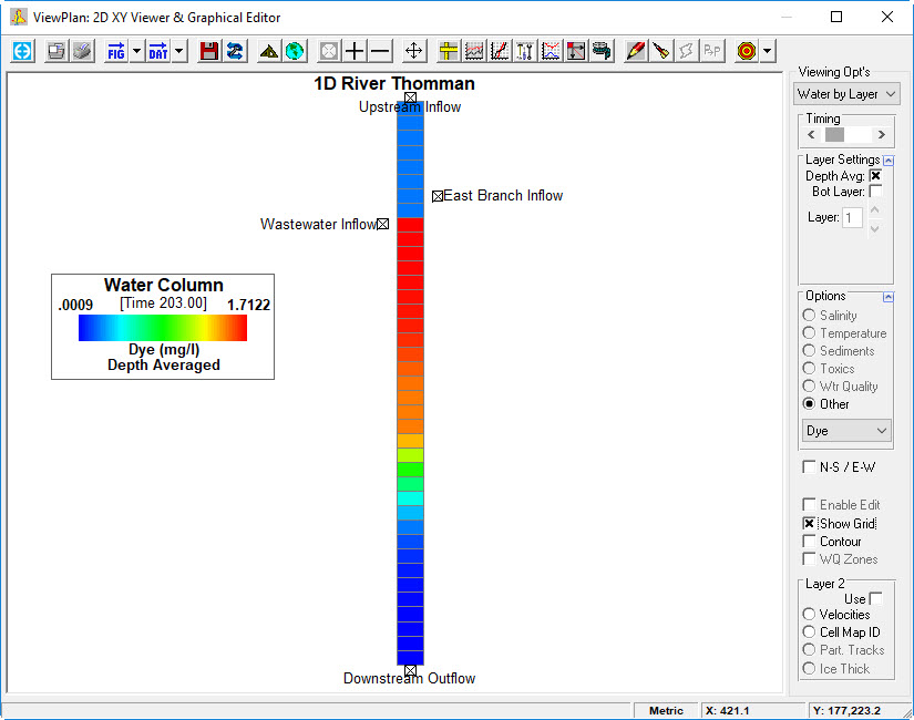
Figure 53  ViewPlan – Water by Layer: dye.

A time series of the dye at that cell will be displayed as shown in Figure 54.

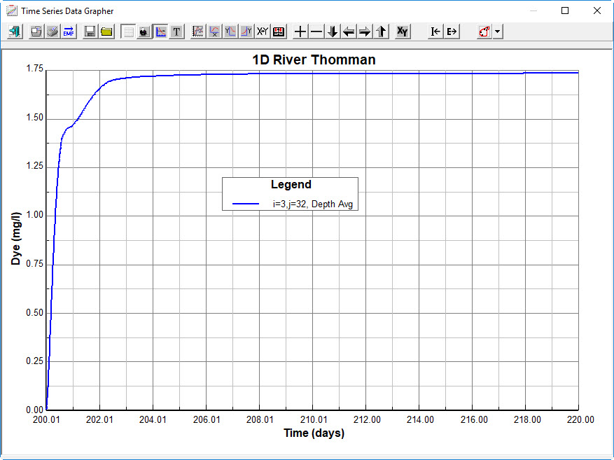
Figure 54  Time series data grapher: dye.

7  Model Calibration Tools

7.1 Profile Plots

A profile plot may be set up using the Longitudinal Profile button in Figure 55

1. Click the Longitudinal Profile button and set I=3.
2. Set Line 1 to 1 to display dye as shown in Figure 55

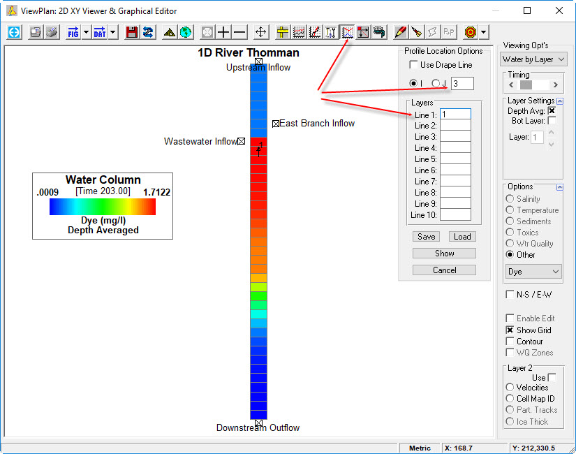
Figure 55  Time series data grapher.

   3. Select Show to display the Profile as shown in Figure 55

   4. Load the comparison file with the Import button shown in Figure 56.

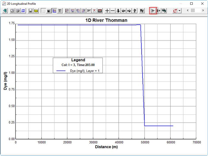
Figure 56 Time series data.

In order to compare to measured data we will create a file of the measured values at RIV01, RIV02 and RIV03 at time = 218 these are shown in Figure 57.

Figure 57  Dye concentration at Time = 218.

   5. Navigate to the .dat file containing the data as shown in Figure 58.

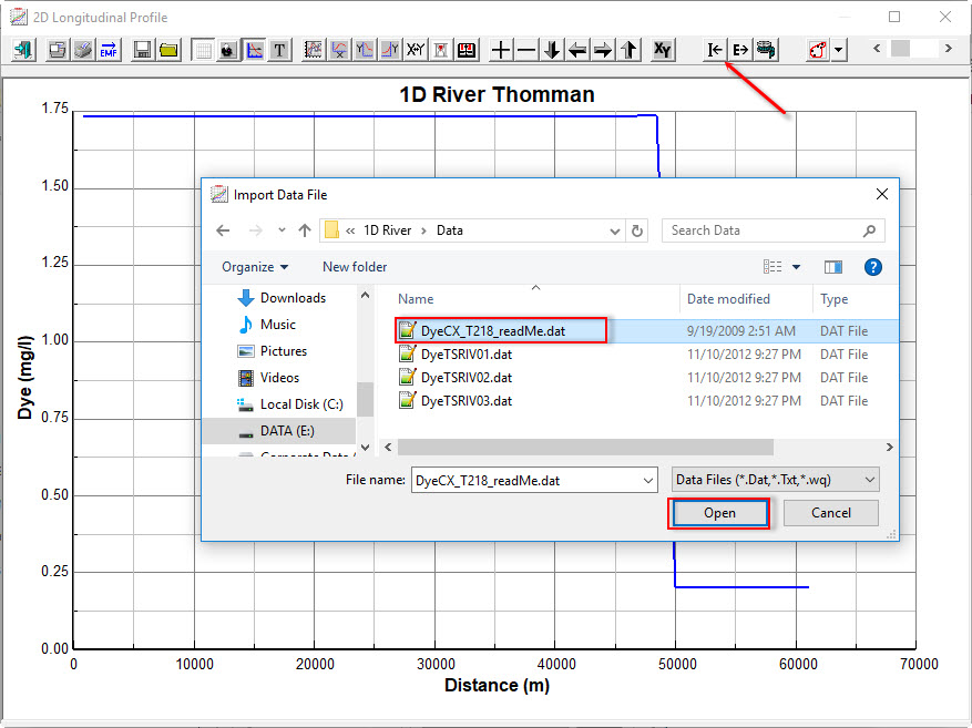
Figure 58  Loading measured data file (1).

   6. If asked if the X values are dates select “No” as shown in Figure 59.

Figure 59  Loading measured data file (2).

   7. Select value = 2 for the series to import the value into (modeled dye is series 1) as shown in Figure 60.

Figure 60  Enter value for timeseries data imported.

   8. RMC on the legend to set the series line options for the data to dots using line plotting options as shown in Figure 61.

   9. Scroll through the timing bar or use CTRL-G to go to t=218 for comparison as shown in Figure 62.

Figure 61  Line plotting options.

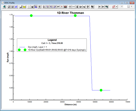
Figure 62  Dye concentration at Time = 218.

7.2 Non-Conservative Substance

To compare with the theoretical results it is necessary to reset the dye as a non-conservative substance as shown below. 

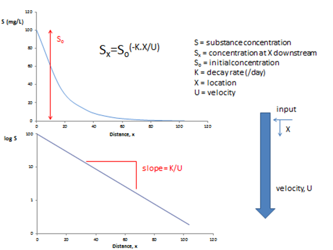
Figure 63  Decay of Non-conservative substances in Cartesian coordinates and Logarithmic form.

1. Set Dye decay to 0.15 as shown in Figure 64.
2. Save the model
3. Run the model

The resulting longitudinal profile will be like that as shown in Figure 65.

Figure 64  Main Form – Dye: dye decay rate.

Figure 65  ViewPlan- Longitudinal Profile: K=0.15 Non-conservative dye.

7.3 Calibrating the Non-conservative Substance

Use the data from Figure 66 (provided in the file “River1D-ExactSolution.dat”) as calibration data for this project

1. As described in Section 7.1 above, load the calibration data with the “I” (Import) button from the from shown in Figure 56.
2. Select No for the question are the X values dates.
3. Select “2” for the value for analytical solution.
4. Use CTRL G to go to time = 218

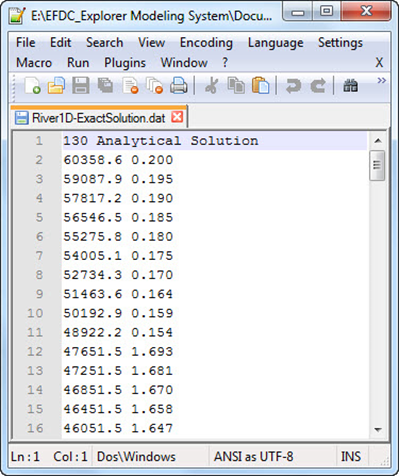
Figure 66  Calibration Data.

Figure 67  Dye Tracer:  comparison of EFDC & analytical solution.

We will now compare measured data at the three station, RIV01, RIV02 and RIV03 described earlier (Figure 31). Data for these stations is as shown below in Figure 68 and contained in the files: DyeTSRIV01.dat, DyeTSRIV02.dat, DyeTSRIV03.dat.

   5. Return to Main Form | Model Analysis | Model Calibration | Time Series Comparisons tool as shown in Figure 69

   6. Click Define/Edit

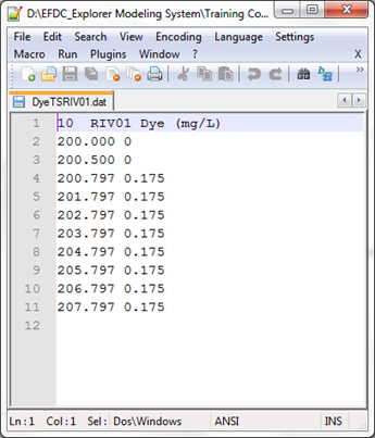
Figure 68  RIV01 calibration data.

Figure 69  Main Form – Model Analysis: model calibration.

   7. Set the Number of time series to 3 as shown in Figure 70

   8. Define the X, Y value for the calibration station for each of the three stations.

   9. Set the K (layer value) to 1 for all stations

   10. Set the ID as RIV01, RIV02 and RIV03

   11. Set the Pathname to the data files

   12. Set Param to 3 for all stations. The full list of parameters available can be seen by pressing F2.

   13. Set R Ave to 0; Set Group to 1, 2, and 3 respectively.

   14. Set Use to 1 for all stations so they are all on.

   15. Click OK

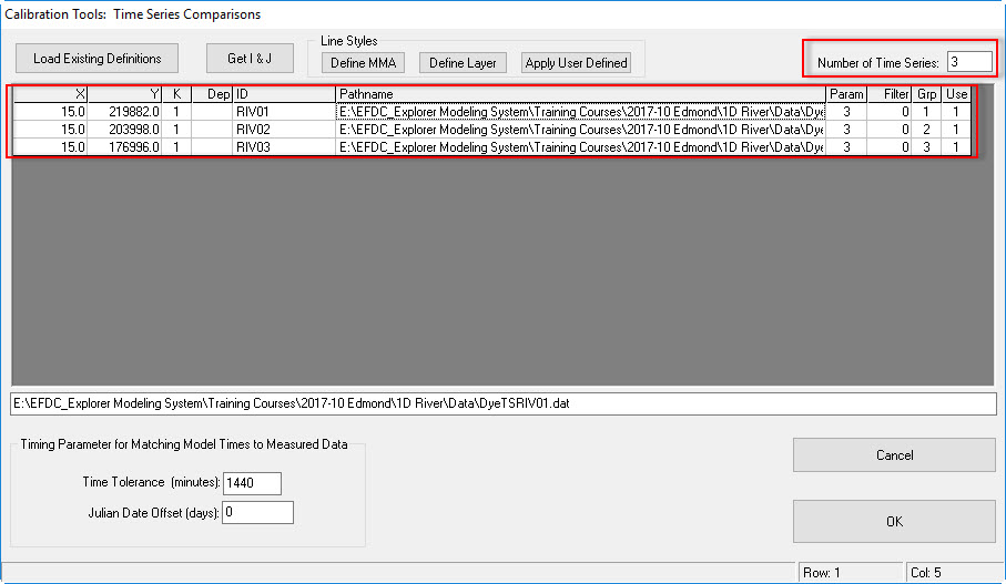
Figure 70  Calibration Tools – time series comparisons.

   16. Click OK for Calibration Plot Generation Options without selecting the checkboxes to display the graph in Figure 71.

We now want to set the data display so that is similar to that shown in Figure 71.

   17. RMC the legend

   18. Select the data series and adjust the settings as shown in Figure 68

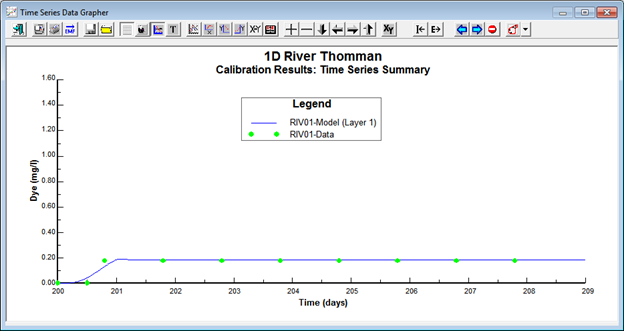
Figure 71  Calibration – time series comparisons: RIV01.

   19. Click Save to save the plot settings shown in Figure 72

Figure 72  Calibration – time series comparisons: line options and controls.

   20. Press the blue arrow key at the top of the data grapher to proceed to the next plot

   21. Load the previously saved Line Options and Controls settings with Load button to apply to the next plot so that it appears as shown in Figure 73.

   22. Apply the above step for RIV03 as shown in Figure 74.

Figure 73  Calibration – time series comparisons: RIV02.

Figure 74  Calibration – time series comparisons: RIV03.