...
In the model interface, click on the Save button to save the model, as shown in Figure 10 below.
| Anchor | ||||
|---|---|---|---|---|
|
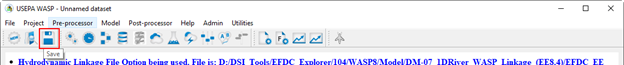
Figure 10. Save Button in the Model Interface.
After the model has been saved, the Executable button will now be enabled. Click on the Executable button to start run the WASP model, and the runtime simulation interface will be displayed as shown in Figure 11 below.
| Anchor | ||||
|---|---|---|---|---|
|
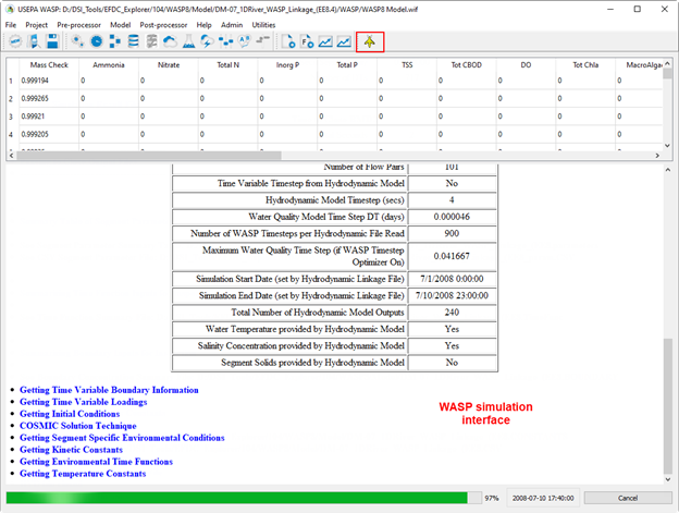
Figure 11. WASP model run interface.
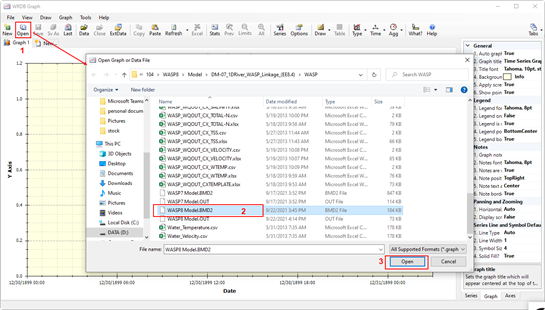
Wait until the model run finishes, then click on the WRDB Graph button from the toolbar for the post-processing.
...
(3) Click the OK button (Figure 12).
| Anchor | ||||
|---|---|---|---|---|
|

Figure 12. Open WASP output from WRDB Graph.
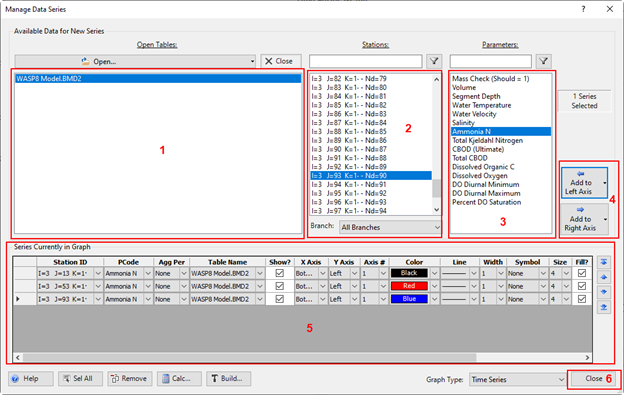
After the Manage Data Series form is displayed:
...
(6) Click the Close button to close the form and plot the output series (Figure 13).
| Anchor | ||||
|---|---|---|---|---|
|
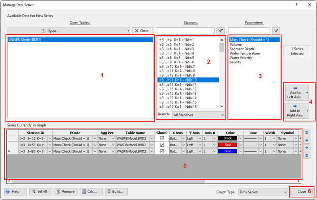
Figure 13. Manage data series to plot.
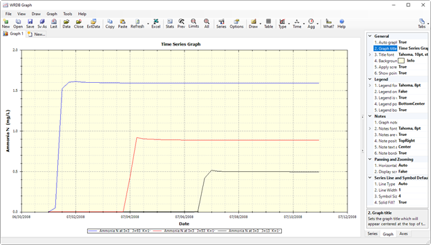
The mass check data time series will be plotted as shown in Figure 14 below.
| Anchor | ||||
|---|---|---|---|---|
|
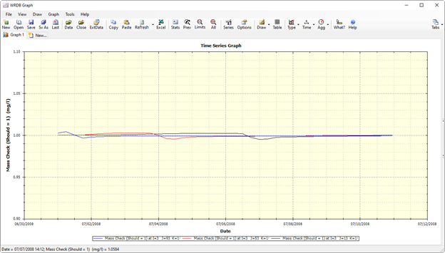
Figure 14. Data series plotted by WRDB Graph.
As shown in Figure 14, the mass check concentration of the segments approaches 1.0 mg/L. It means the simulation is run for a sufficient duration and reaches to steady state.
Figure 3-xx 15 shows a comparison of the water velocity in WASP and EFDC at cell yy. The two curves are almost identical, provide verification of the flow information from the hydrodynamic linkage.
| Anchor | ||||
|---|---|---|---|---|
|
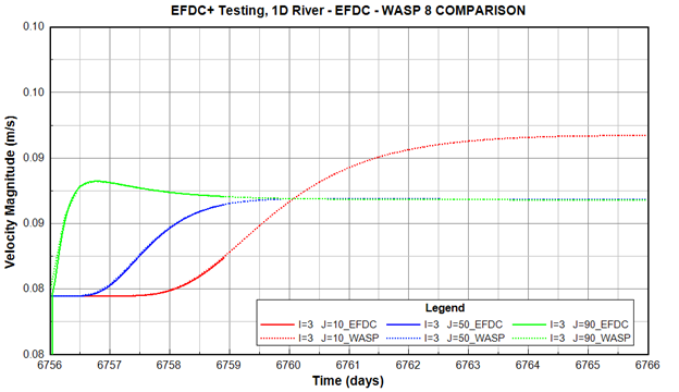
Figure 15. EFDC+ and WASP 8 velocity Comparison.
Building WASP water quality model
...
(4) Click the OK button to save settings (Figure 16)
| Anchor | ||||
|---|---|---|---|---|
|
|
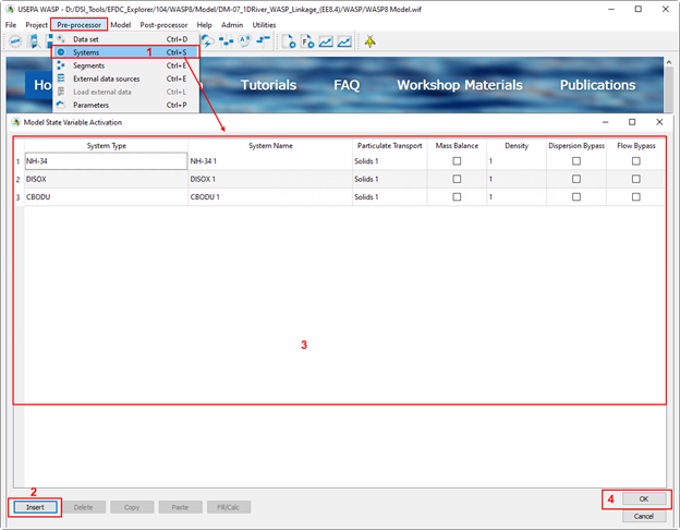
Figure 16. Add water quality constituents to the WASP model.
After adding water quality constituents to the WASP model, we will now add the boundary condition in the next step. From the WASP interface, go to Pre-processor\Boundary Condition and Loads as shown in Figure 17 below.
| Anchor | ||||
|---|---|---|---|---|
|
|
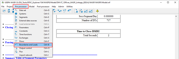
Figure 17. Add water quality boundary conditions to WASP model.
From Boundaries and Loads form, under Boundaries tab
...
(3) After filling the data series for all boundaries, click OK to save the boundary data (Figure 18).
| Anchor | ||||
|---|---|---|---|---|
|
|
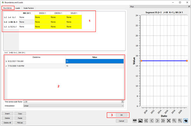
Figure 18. Add water quality boundary conditions data series.
After the boundary conditions have been added, we will set the model parameters and kinetic coefficients for the model.
From the WASP interface, go to Pre-processor\Constants as shown in Figure 19.
| Anchor | ||||
|---|---|---|---|---|
|
|
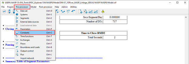
Figure 19. Set model parameters and kinetic coefficients.
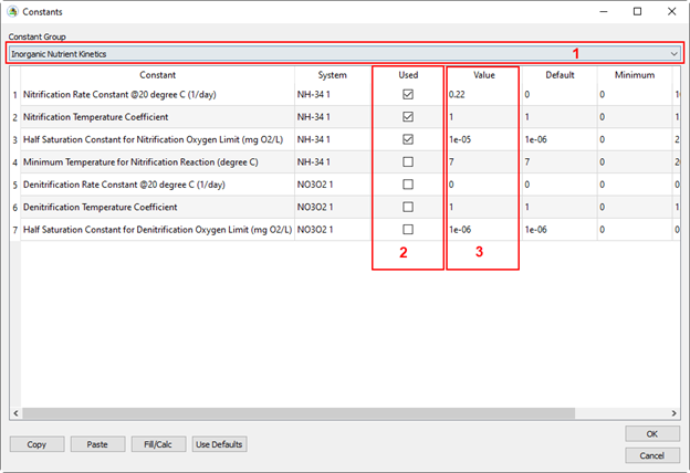
From Constants form,
(1) Select the constant group;
...
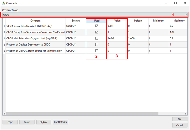
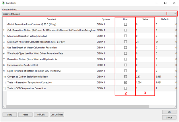
(3) Set the parameter values for constant groups as shown in Figure 3‑20 20 to Figure 3‑2323;
| Anchor | ||||
|---|---|---|---|---|
|
|
Figure
...
20. Set Inorganic Nutrient kinetics parameters.
| Anchor | ||||
|---|---|---|---|---|
|
|
Figure
...
21. Set CBOD parameters.
| Anchor | ||||
|---|---|---|---|---|
|
|
Figure
...
22. Set dissolved oxygen parameters.
| Anchor | ||||
|---|---|---|---|---|
|
|
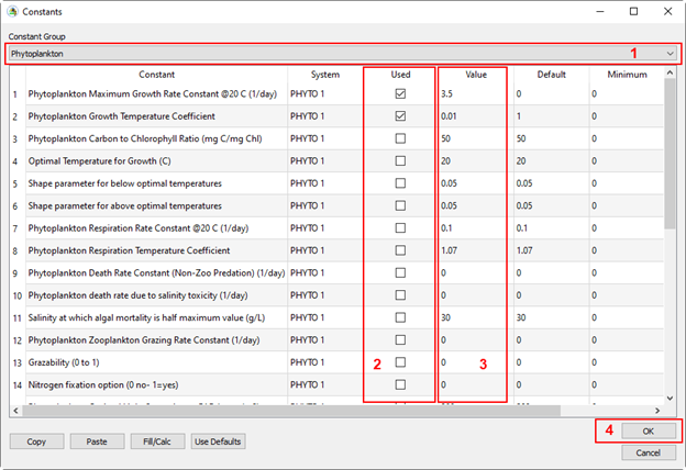
Figure
...
23. Set Phytoplankton parameters.
(4) Click OK button to save settings after set the kinetic parameters as shown in Figure 3‑2223;
After set the model parameters, from toolbar, click on the Output Control button to open Output Control form and add the water quality constituents to the output as shown in Figure 3‑2424.
| Anchor | ||||
|---|---|---|---|---|
|
|

Figure
...
24. Set Output Control.
From the Output Control form,
...
(2) Check on the checkbox corresponding to the parameter will be written out as shown in Figure 3‑25 25 to Figure 3‑2727;
| Anchor | ||||
|---|---|---|---|---|
|
|
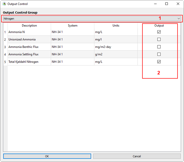
Figure
...
25. Add Nitrogen parameters to the output.
| Anchor | ||||
|---|---|---|---|---|
|
|
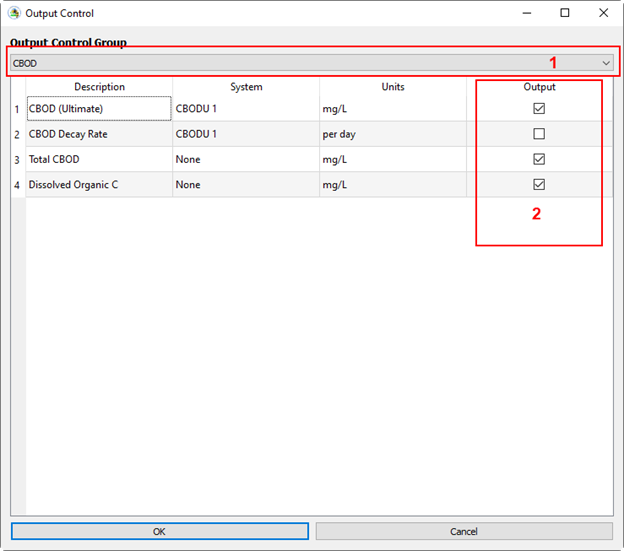
Figure
...
26. Add CBOD parameters to the output.
| Anchor | ||||
|---|---|---|---|---|
|
|
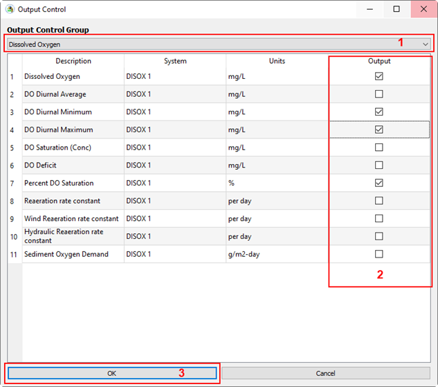
Figure
...
27. Add DO parameters to the output.
(3) Click the OK button to save settings as shown in Figure 3‑2727;
After finishing the settings for the model, from the toolbar,
- Save the model;
- Run WASP model as shown in Figure 3‑2828
| Anchor | ||||
|---|---|---|---|---|
|
|

Figure
...
28. Save and run WASP model.
Visualize WASP Output
Wait for the model run finish, then go to WRDB Graph to check the model output as we did for checking hydrodynamics output before.

The WRDB Graph window now appears, from WRDB Graph window,
...
(3) Click the OK button (Open WASP output from WRDB GraphFigure 3‑29Graph Figure 29).
| Anchor | ||||
|---|---|---|---|---|
|
|
Figure
...
29. Open WASP output from WRDB Graph.
Manage Data Series form appears, from here
...
(6) Click the Close button to close the form and visualize the output series (Figure 3‑3030).
| Anchor | ||||
|---|---|---|---|---|
|
|
Figure
...
30. Manage data series to plot.
The data series will be plotted as shown in Figure 3‑31 31 below.
| Anchor | ||||
|---|---|---|---|---|
|
|
Figure
...
31. Data series plotted by WRDB Graph.
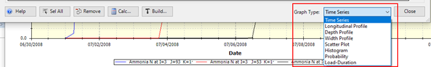
Note: In the bottom right corner of the Manage Data Series form, the Graph Type frame is available to allow the user to view the output in different ways, as shown in Figure 3‑32 32 below.
| Anchor | ||||
|---|---|---|---|---|
|
|
Figure
...
32. Graph type of WRDB Graph.
For graph types like Longitudinal Profile, Depth Profile, for which the value change by time, the timing bar is available in the bottom of the WRDB Graph window (Figure 3‑3333). Therefore, the user can move the time or run animation to see how the output changes in a profile.
| Anchor | ||||
|---|---|---|---|---|
|
|
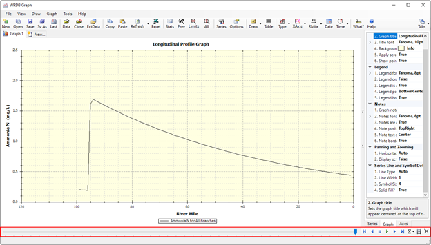
Figure
...
33. Timing bar in Longitudinal Profile Graph.
After the output graphs have been plotted, from toolbars, the user can select Send data and graph to Microsoft Excel button to extract data then import as external data to EE to compare the output between WASP and EFDC+.
Some output comparison graphs are shown in Figure 3‑34 34 to Figure 3‑38 38 below.
| Anchor | ||||
|---|---|---|---|---|
|
|

Figure
...
34. Time series comparison of water temperature between EFDC+ and WASP output.
| Anchor | ||||
|---|---|---|---|---|
|
|

Figure
...
35. Time series comparison of DO between EFDC+ and WASP output.
| Anchor | ||||
|---|---|---|---|---|
|
|
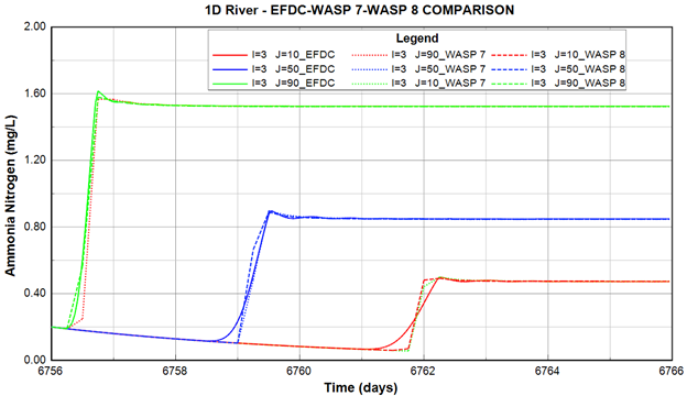
Figure
...
36. Time series comparison of NH3-N between EFDC+ and WASP output.
| Anchor | ||||
|---|---|---|---|---|
|
|
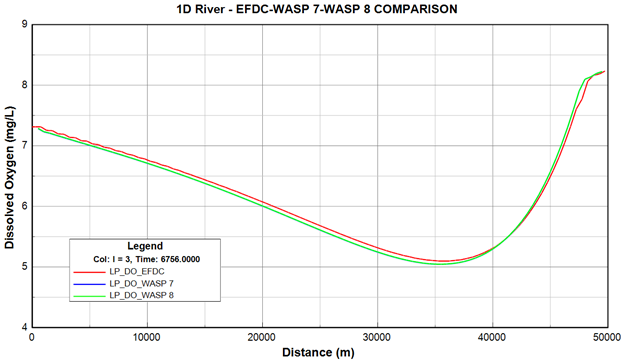
Figure
...
37. Longitudinal profile comparison of DO between EFDC+ and WASP output.
| Anchor | ||||
|---|---|---|---|---|
|
|
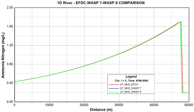
Figure
...
38. Longitudinal profile comparison of NH3-N between EFDC+ and WASP output.