...
(4) Type in 900 to # of Time Periods to Average box to set the output frequency of the linkage file. The output frequency will be calculated by multiply multiplying this value and the time step value. In this case, the model time step is 4 (sec.), so the wasp linkage output will be saved per 1 hour.
...
Figure 2. Save Button in the Model Interface.
After clicking on the Save button, a Select Directory: Write Operation pop-up will appear to select saving options (refer to Figure 3). Before project files are saved, the grey box is empty. This is where EE project files will be listed. The empty gray box shows that no files have been written yet for the study, as shown in Figure 3.
...
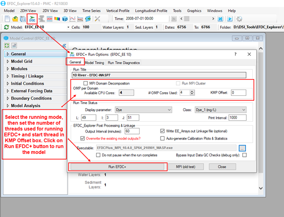
To run the model, follow the steps below, as shown in Figure 3‑44.
Click on the Run EFDC button at the top of the model interface to run the model. The EFDC+ Run Options form will appear; Figure 3‑44. in this form, under the General tab, set the Number of OMP Threads to use for the EFDC+ run in the EFDC+ Multi-Threading frame. Note that the number of threads used for the EFDC+ run must be smaller than the total number of threads.
Also, in the EFDC+ Multi-Threading frame, set the KMP Offset to set the threads that will be passed over when running the model. For example, if KMP Offset is set to 2, that which means the thread used for the EFDC+ run will start from the 3rd thread. This can be used to run multiple models on one machine, so the models run on different threads.
Note: If the model has existing results, please check the Overwrite check box to run and save new results.
| Anchor | ||||
|---|---|---|---|---|
|
|
Figure
...
4. EFDC+ Run Options form.
Click on the Run EFDC+ button to start running the model. A run window such as that pictured in in Figure 3‑5 5 will appear.
| Anchor | ||||
|---|---|---|---|---|
|
...
|
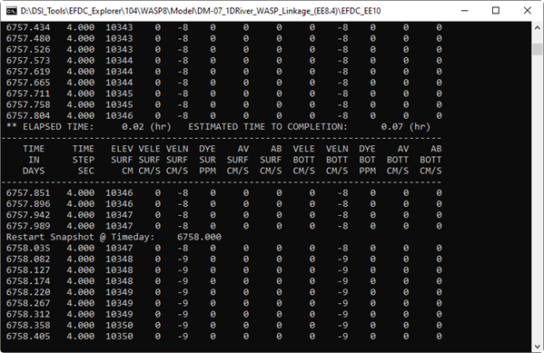
Figure 5. EFDC+ run window.
After the EFDC+ model run is finished, the user should browse to the output folder to make sure that the efdc_dsi_wasp.hyd file has been generated. It should be noted that the WASP8SEG_EFDCIJK.DAT file allows the identification of the corresponding segment between the WASP and the EFDC cell.
| Anchor | ||||
|---|---|---|---|---|
|

Figure 3‑36. Saving the model.
...
WASP Linkage file generated by EFDC+.
Building WASP model with using Hydrodynamics Linkage
From the WASP program interface, click on the New button in the toolbars to create a new project
| Anchor | ||||
|---|---|---|---|---|
|
...
|
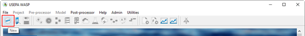
Figure 7. Create a new WASP project.
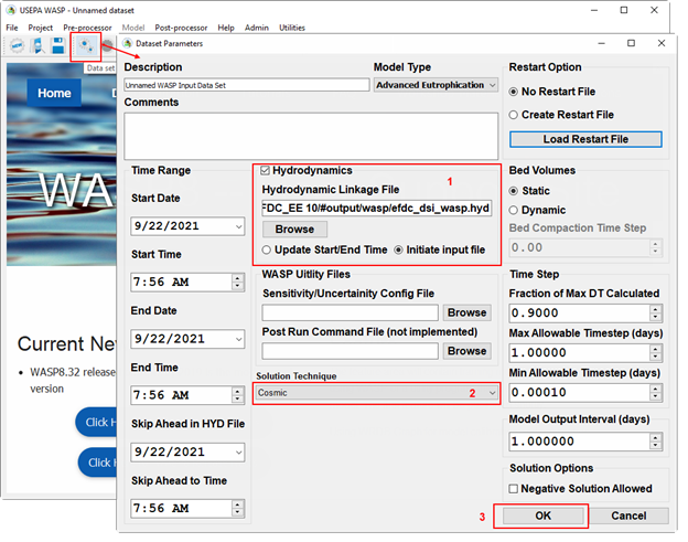
After creating a new project, click on the Data Set button, which is now enabled in the toolbar, then carry out the following steps to link hydrodynamic input:
...
(4) Click the OK button to save the setting (Figure 3‑88).
| Anchor | ||||
|---|---|---|---|---|
|
|
Figure
...
8. Link hydrodynamics output from EFDC+ to WASP model.
The next step when setting up a new WASP is to check at this point if the data provided by EFDC hydrodynamic linkage file are read correctly by WASP8. User can also check the numerical stability of the hydrodynamic linkage by inspecting the “Mass Check” system on the runtime and in model output.
...
(2) Check on the output checkboxes for Mass Check, as well as the transport quantities that user want wants to write out to compare with the EFDC model.
(3) Click the OK button to save the setting (Figure 3‑99).
| Anchor | ||||
|---|---|---|---|---|
|
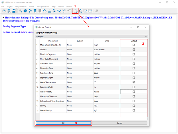
Figure 3‑39. Saving the model.
...
Select WASP output parameter to write out.
In the model interface, click on the Save button to save the model, as shown in Figure 10 below.
| Anchor | ||||
|---|---|---|---|---|
|
Figure 10. Save Button in the Model Interface.
After the model has been saved, the Executable button will now be enabled. Click on the Executable button to start run the WASP model, and the runtime simulation interface will be displayed as shown in Figure 11 below.
| Anchor | ||||
|---|---|---|---|---|
|
Figure 3‑3. Saving the model.
...
11. WASP model run interface.
Wait until the model run finishes, then click on the WRDB Graph button from the toolbar for the post-processing.
...
(3) Click the OK button (Figure 12).
| Anchor | ||||
|---|---|---|---|---|
|
Figure 3‑3. Saving the model.
...
12. Open WASP output from WRDB Graph.
After the Manage Data Series form is displayed:
...
(6) Click the Close button to close the form and plot the output series (Figure 13).
| Anchor | ||||
|---|---|---|---|---|
|
Figure 3‑3. Saving the model.
...
13. Manage data series to plot.
The mass check data time series will be plotted as shown in Figure 14 below.
| Anchor | ||||
|---|---|---|---|---|
|
|
Figure 14. Data series plotted by WRDB Graph.
As shown in Figure 14, the mass check concentration of the segments approaches 1.0 mg/L. It means the simulation is run for a sufficient duration and reaches to steady state.
Figure 3-xx shows a comparison of the water velocity in WASP and EFDC at cell yy. The two curves are almost identical, provides a provide verification of the flow information from the hydrodynamic linkage.
| Anchor | ||||
|---|---|---|---|---|
|
Figure 3‑3. Saving the model.
...
15. EFDC+ and WASP 8 velocity Comparison.
Building WASP water quality model
...