Building a 2D Lake Water Quality Model (Level 2 Step-by-Step Guidance)
1. Introduction
Lake Thonotosassa is the largest natural freshwater lake in Hillsborough County covering an area of 849 acres (3.44 km2) (Hillsborough County Water Atlas). The lake is fed by Baker Creek at the southeastern end of the lake and water flows out through Flint Creek on the northeastern end to the Hillsborough River (Figure 1). This guidance document carries on from the hydrodynamic model introduced in Build a 2D Lake Model (Level 1 Step-by-Step Guidance). The model files are contained in the Demonstration Models of the Resources page folder file (DM-14 Lake T Hydrodynamic and WQ Model).
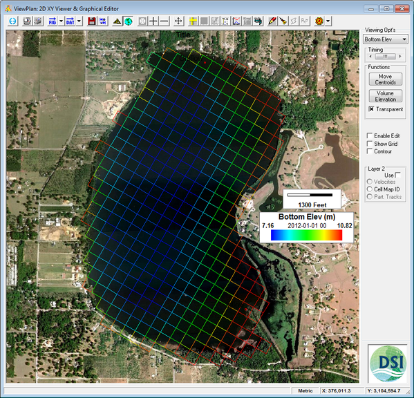
Figure 1 Lake Thonotosassa location map.
2. Description of Hydrodynamic Model
This model is used as the basis for building a water quality model that is part of this guidance document. Figure 2 provides a representation of the digital terrain model for Lake Thonotosassa. All of the boundary types for the Lake Thonotosassa model are flow boundaries, the locations of flow boundary conditions are presented in Figure 3. Flow discharge and temperature used for the model are shown in Figure 4. Figure 5 shows a wind rose of the wind data.
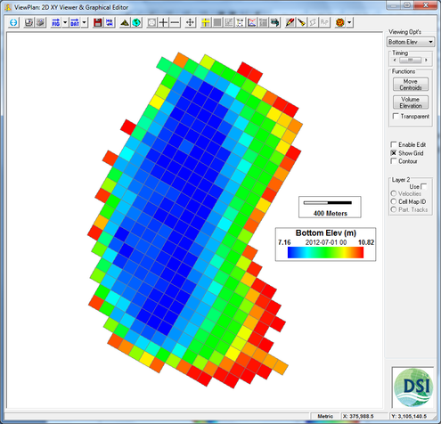
Figure 2 EFDC model bathymetry Lake Thonotosassa.
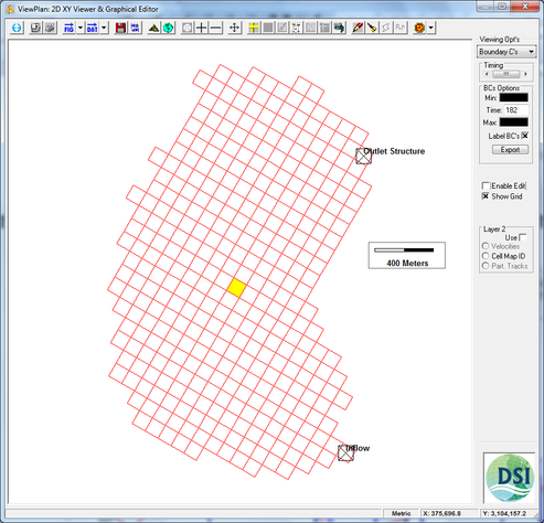
Figure 3 Boundary condition map Lake Thonotosassa.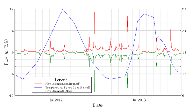
Figure 4 Flow and Temperature boundary conditions.
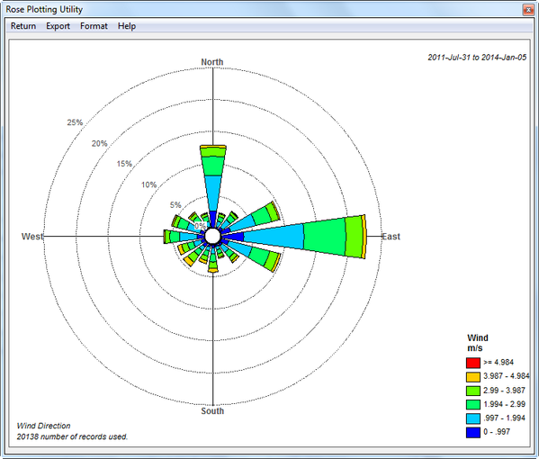
Figure 5 Winds boundary conditions.
3. Setting Water Quality Model
Open the hydrodynamic model then add wind data in the model as shown in Figure 6.
In the Main Form of EE click the Edit (E) button for Winds to edit the winds boundary. Enter the Number of Series into the box. There are one winds boundary so it should be “1”.
Give a Title for associated time series. In this case, title “winds” for Current series 1.
Copy and Paste time series data, “Winds.dat,” into the workspace corresponding to the winds as shown in Figure 7 then click OK button.
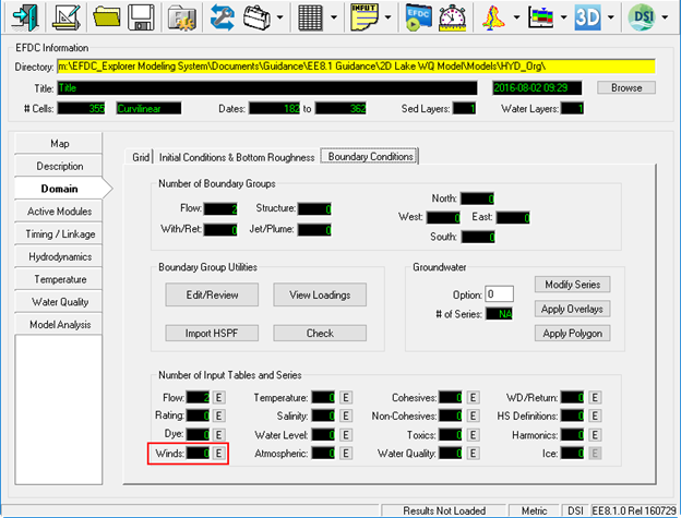
Figure 6 Open Hydrodynamic model.
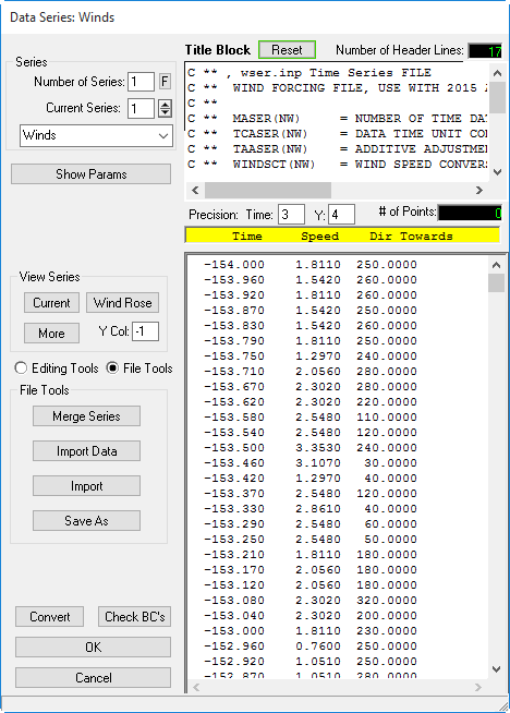
Figure 7 Assign Winds BC.
In the Main Form of EE, select Active Modules tab and turn on the "Temperature and Water Quality" module as shown in Figure 9.
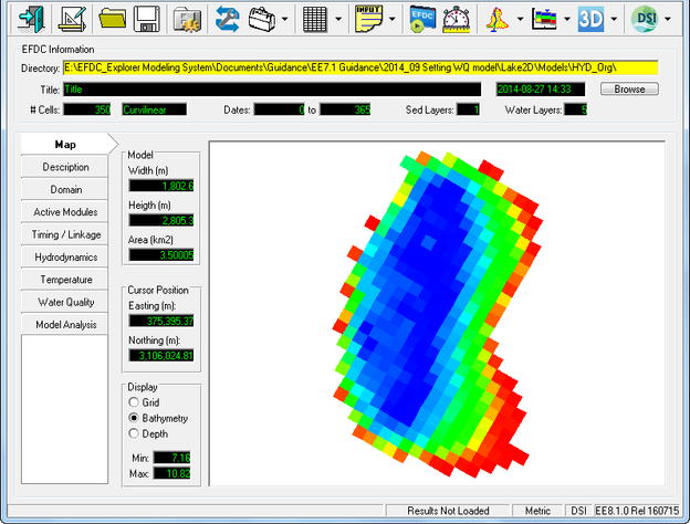
Figure 8 Open Hydrodynamic model.
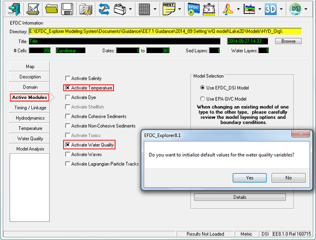
Figure 9 Activate Temperature and Water Quality.
After the check box for Activate Water Quality is enabled, a prompt from EE ask if we want to initialize default values for the WQ variables as shown in Figure 10.
Note that from EE7.3 and later we have the efdc.mdb file, which contains the default values for WQ. This saves the user a lot of time as they no longer need to manually enter these values. If they say "No" they have to manually enter the values or import them from a previous model.
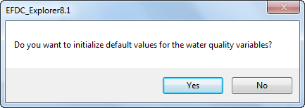
Figure 10 Yes/No to Initialize default values for WQ variables.
3.1 Create the temperature boundary time series; the atmospheric boundary time series and set IC for temperature
1. Proceed to the Temperature tab shown in Figure 11. From this form we can create the temperature boundary time series and the atmospheric boundary time series
2. Select the I for Edit button on Temperature for the Time series Data. This will display the form shown in Figure 12
3. Set the number of flow series to 1; current series 1
4. Set the title to "Temp Inflow" and type or copy and paste into the form for the time and temperature data (Figure 13)
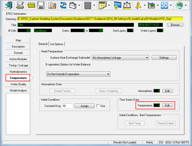
Figure 11 Main Form – Temperature Settings.
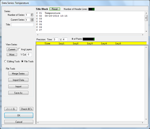
Figure 12 Boundary Condition Settings: Temperature Data Series.
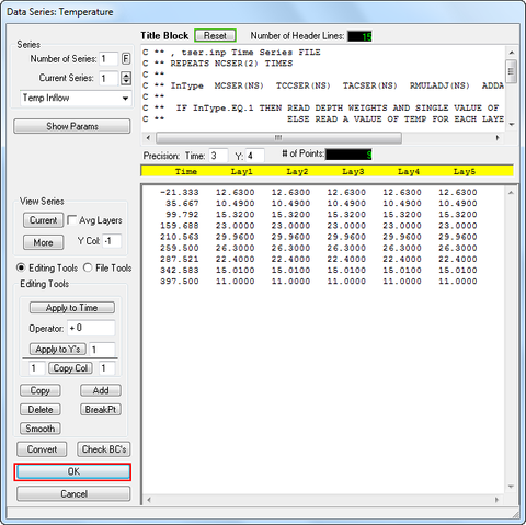
Figure 13 Boundary Condition: Temperature Inflow.
5. Return for the Main Form shown in Figure 9 and select the E button for Atmospheric
6. Repeat the above process for atmospheric data as shown in Figure 14
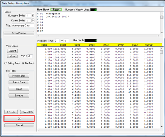
Figure 14 Boundary Condition: Atmospheric data.
7. Click OK button to return for the Main Form shown in Figure 11. In the Heat/Temperature frame LMC to Surface Heat Exchange Submodel box, the drop down list provides several options, including Atmospheric linkage, Full Heat Balance, External Equilibrium Temperature, Constant Equilibrium Temperature and Equilibrium temperature (CE-QUAL-W2 method, EFDC_DSI only). Select Equilibrium Temp (CE-QUAL-W2 method) as shown in Figure 15.
8. In the Main Form shown Figure 11 then select the Settings button in the Heat/Temperature frame. When pressed, the form shown in Figure 16 is displayed, type in the atmospheric parameters into the Value column then click Ok button.
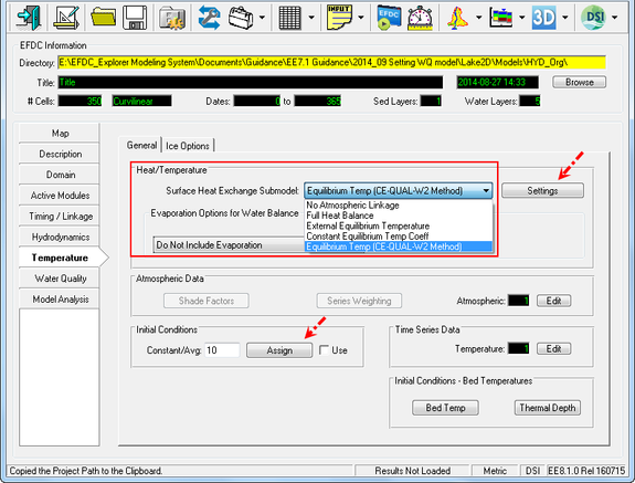
Figure 15 Select type of Surface Heat Exchange Submodel.
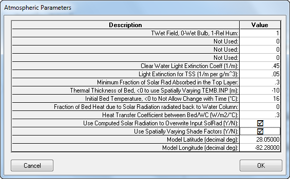
Figure 16 Atmospheric Parameters.
9. Select the Assign button for temperature to display the form shown in Figure 17
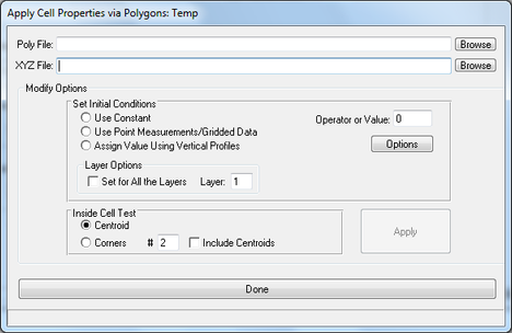
Figure 17 Assigning IC for Temperature.
10. Select Use Constant from the Set Initial Conditions and set Operator = 10.5. In the Layer Options frame select Set for All the layers or do not select to set for each layer Figure 18
11. Select Apply and Done to apply these changes. EE will tell you that this has been applied to 349 cells which is all the cells in the domain.
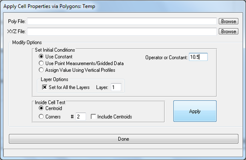
Figure 18 Assigning IC for model domain.
3.2 Create the Water Quality time series and set Initial Water quality
3.2.1 Water Quality – Kinetics
1. Proceed to the The "WQ - Kinetics" tab, select Module 1 (Standard) from the Global Kinetic Options frame drop down is shown in Figure 19.
2. Click the Params button display the list of parameters simulated; type 1 for parameter simulated and 0 for not simulated as shown in Figure 20.
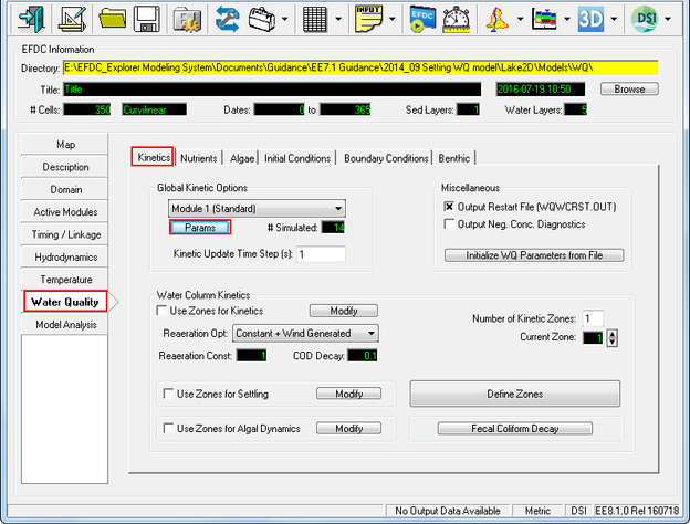
Figure 19 Water Quality Tab: Kinetics.
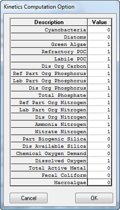
Figure 20 Kinetics Computation Option.
3. Click Modify button in the frame Water Column Kinetics | Use Zones for Kinetics to edit Parameter for current zone as shown in Figure 21.
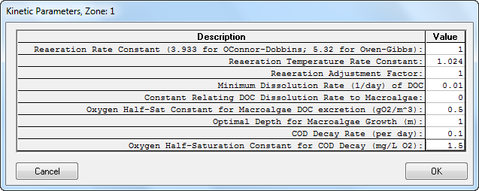
Figure 21 Kinetics Parameters for zone.
4. Click Modify button in the frame Water Column Kinetics | Use Zones for Algal Dynamics to edit Parameter for current zone as shown in Figure 22.
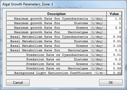
Figure 22 Algal Growth Parameters.
5. Click Fecal Coliform Decay button in the frame Water Column Kinetics to edit Parameter for current zone as shown in Figure 23.
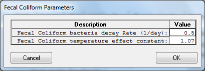
Figure 23 Fecal Coliform Parameters.
3.2.2 Water Quality – Nutrients
Proceed to the The "WQ - Nutrients" tab; The "WQ - Nutrients" tab is shown in Figure 24. Within the "Nutrient Options and Parameters" frame click Carbon button to edit the Carbon parameters Figure 25; Nitrogen button to edit the Nitrogen parameters Figure 26; Phosphorus button to edit the Phosphorus parameters Figure 27; COD&DO button to edit the COD&DO parameters Figure 28.
In the Sorption Option select Total Active Metal (TAM) Based then click Modify Parameters buttons to edit Nutrient Sorption Parameters Figure 29.
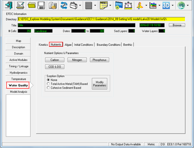
Figure 24 Water Quality Tab: Nutrients.
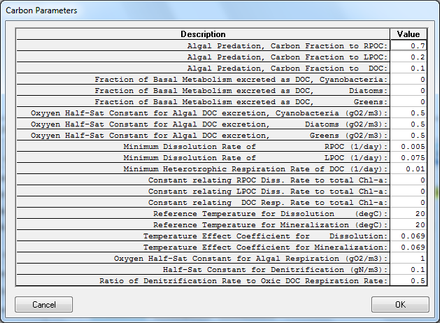
Figure 25 Nutrients: Carbon Parameters.
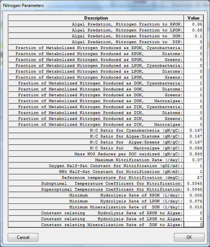
Figure 26 Nutrients: Nitrogen Parameters.
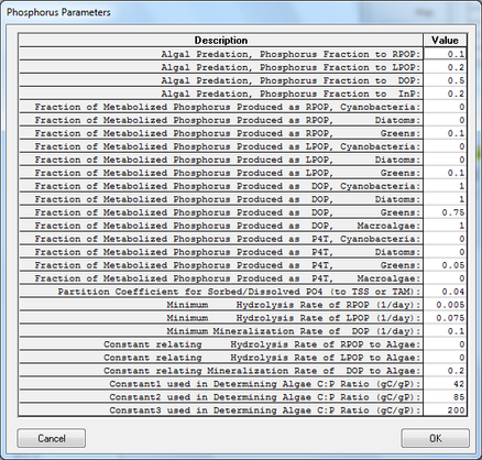
Figure 27 Nutrients: Phosphorus Parameters.
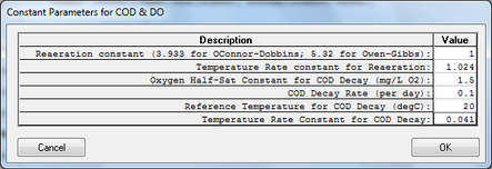
Figure 28 Nutrients: COD and DO Parameters
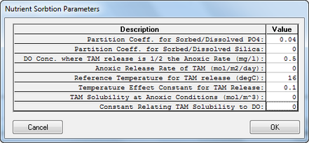
Figure 29 Nutrients: Nutrient Sorption Parameters.
3.2.3 Water Quality – Algae
Proceed to the The WQ - Algae tab; The WQ - Algae tab is shown in Figure 30; Within the Solar Radiation for Algae frame click Modify button to edit the solar radiation parameters shown in Figure 31.
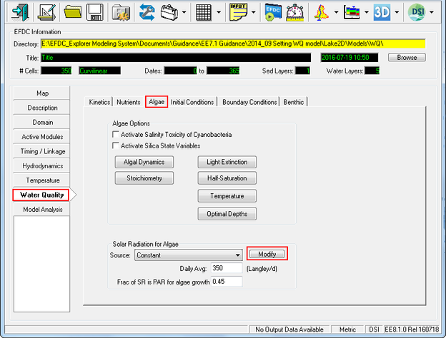
Figure 30 Water Quality Tab: Algae.
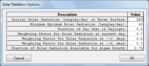
Figure 31 Solar Radiation Options.
3.2.4 Water Quality – Initial Conditions
Proceed to the The WQ – Initial Conditions tab; The WQ – Initial Conditions tab is shown in Figure 32. Within the Initial Conditions frame click Const IC's button to edit each of the water quality parameters Figure 33.
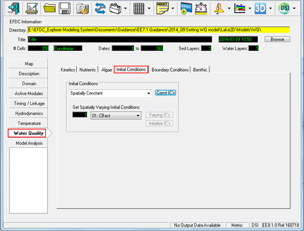
Figure 32 Water Quality Tab: Initial Conditions.
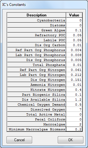
Figure 33 Initial Conditions Parameters.
3.2.5 Water Quality – Boundary Conditions
1. Proceed to the The WQ – Boundary Conditions tab; The WQ – Initial Conditions tab is shown in Figure 34; Click Edit button in the Time series Data frame. This will display the form shown in Figure 35.
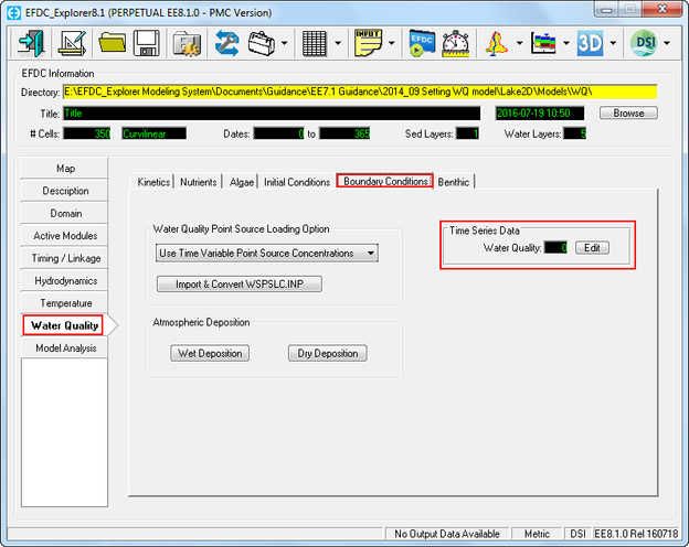
Figure 34 Water Quality Tab: Boundary Conditions.
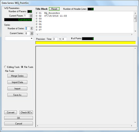
Figure 35 Boundary Condition Settings: WQ Data Series.
2. Set the number of series to 1; Use the arrow buttons below to go to series 1. Set the title to "WQ Data" and type or copy and paste into the form for the time and Cyanobacteria data as shown in figure 36 .
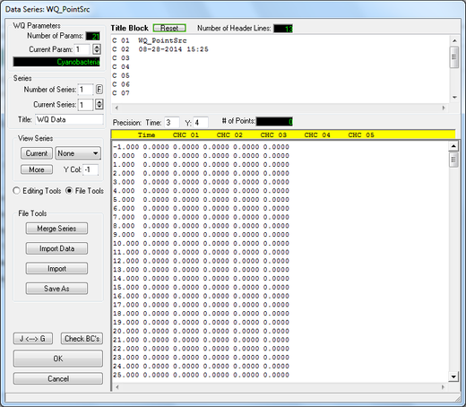
Figure 36 Boundary Condition Settings: Cyanobacteria Data Series.
3. Use the arrow buttons in the Current Param box to go to others parameters appear message from EE shown in Figure 37. Click Yes button to apply changes across all parameters or click No to don't apply all.
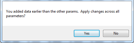
Figure 37 Message from EE.
4. Copy and paste into the form for the time and diatom algae data as shown in Figure 38
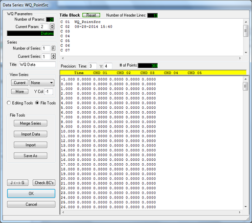
Figure 38 Boundary Condition Settings: Diatom algae Data Series.
5. Repeat this process for the others parameters in the list below
3) Green algae | Figure 39 | 13) Dissolved organic nitrogen | Figure 49 |
4) Refractory particulate organic carbon | Figure 40 | 14) Ammonia nitrogen | Figure 50 |
5) Labile particulate organic carbon | Figure 41 | 15) Nitrate nitrogen | Figure 51 |
6) Dissolved carbon | Figure 42 | 16) Particulate biogenic silica | Figure 52 |
7) Refractory part. organic phosphorus | Figure 43 | 17) Dissolved available silica | Figure 53 |
8) Labile particulate organic phosphorus | Figure 44 | 18) Chemical oxygen demand | Figure 54 |
9) Dissolved organic phosphorus | Figure 45 | 19) Dissolved oxygen | Figure 55 |
10) Total phosphate | Figure 46 | 20) Total active metal | Figure 56 |
11) Refractory part. Org. nitrogen | Figure 47 | 21) Fecal coliform bacteria | Figure 57 |
12) Labile part. organic nitrogen | Figure 48 |
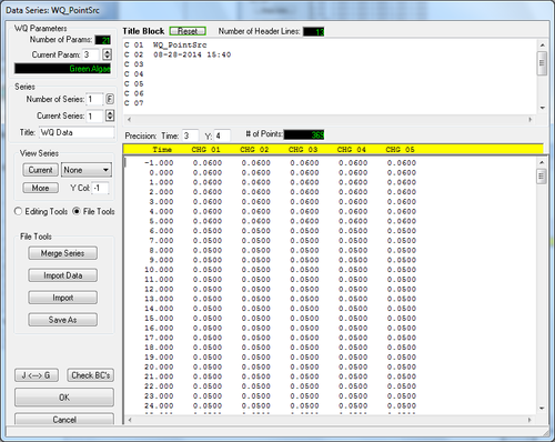
Figure 39 Boundary Condition Settings: green algae.

Figure 40 Boundary Condition Settings: Refractory particulate organic carbon.
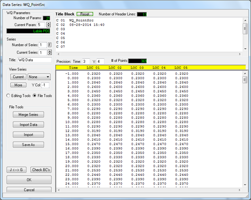
Figure 41 Boundary Condition Settings: Labile particulate organic carbon.

Figure 42 Boundary Condition Settings: DOC.
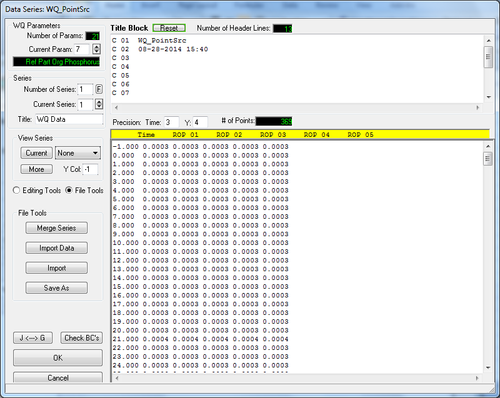
Figure 43 Boundary Condition Settings: Refractory particulate organic phosphorus.
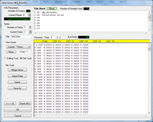
Figure 44 Boundary Condition Settings: Labile particulate organic phosphorus.

Figure 45 Boundary Condition Settings: Dissolved organic phosphorus.

Figure 46 Boundary Condition Settings: Total phosphate.

Figure 47 Boundary Condition Settings: Refractory particulate organic nitrogen.

Figure 48 Boundary Condition Settings: Labile particulate organic nitrogen.

Figure 49 Boundary Condition Settings: Dissolved organic nitrogen.

Figure 50 Boundary Condition Settings: Ammonia nitrogen.
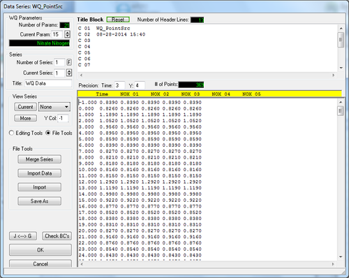
Figure 51 Boundary Condition Settings: Nitrate nitrogen.
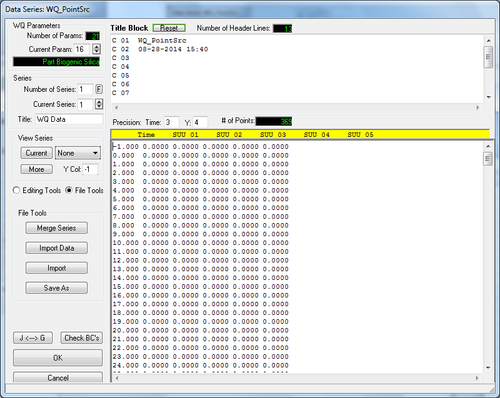
Figure 52 Boundary Condition Settings: Particulate biogenic silica.
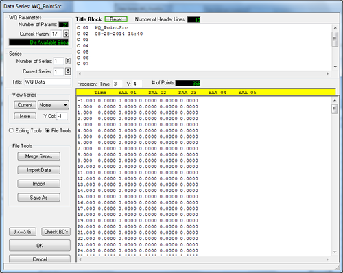
Figure 53 Boundary Condition Settings: Dissolved available silica.
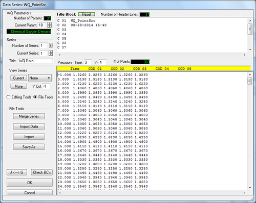
Figure 54 Boundary Condition Settings: Chemical oxygen demand.
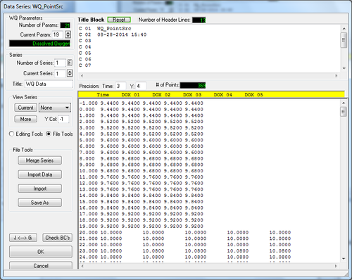
Figure 55 Boundary Condition Settings: Dissolved oxygen.

Figure 56 Boundary Condition Settings: Total active metal. 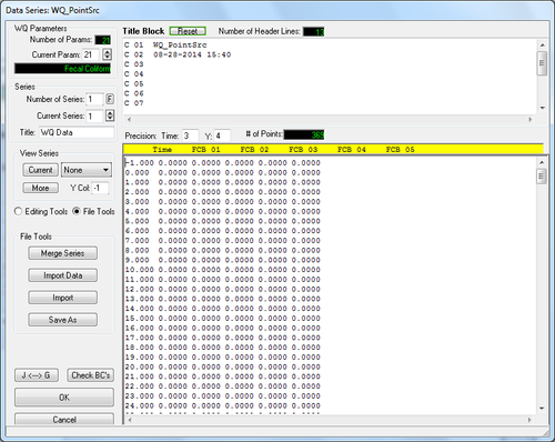
Figure 57 Boundary Condition Settings: Fecal coliform bacteria.
6. Click OK button when finished set 21 parameters
3.2.6 Water Quality – Benthic
1. Proceed to the Water Quality Tab/ Benthic sub tab shown in Figure 58
2. Select the Modify Parameters button will now be displayed Sediment Diagenesis Option & Parameters as shown in Figure 59.
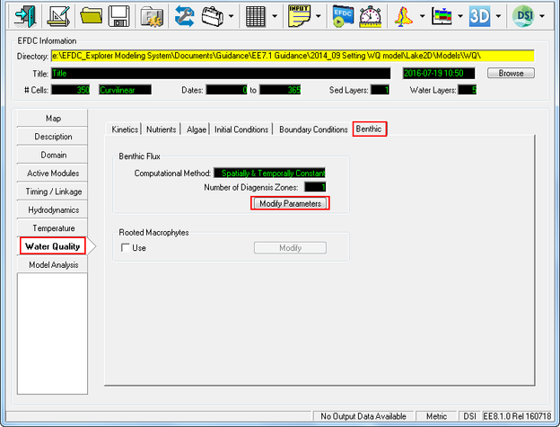
Figure 58 Water Quality Tab: Benthic.
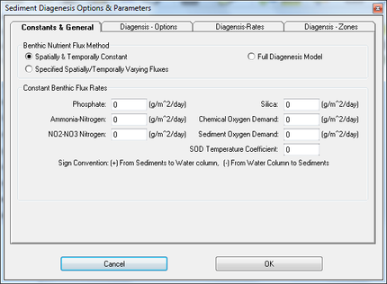
Figure 59 Sediment Diagenesis Option & Parameters.
3. From Sediment Diagenesis Option & Parameters form (Figure 59), in the top frame, Benthic Nutrient Flux Method select Spatially & Temporally Constant; enter the values of parameters in the Constant Benthic Flux Rates frame as shown in Figure 60.
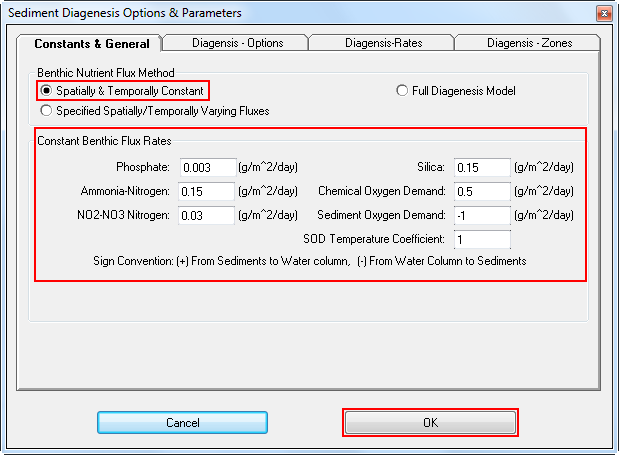
Figure 60 Set Benthic Flux Rates.
4. Click OK button when finish set to return to main form
3.2.7 Linking the time series to the BC locations
1. Select ViewPlan: 2D Plan of Grid & Data
2. Select View Initial Conditions Figure 61
3. To link the time series with the BC locations, Select Boundary Conditions from the Viewing Options drop down. Select Enable Edit. RMC on the location of Inflow BC and select Edit Figure 62.
4. The Modify/Edit BC Properties will now be displayed. This form is used to link the Temperature and Water Quality table to the BC.
5. Set the Concentration tables | Temperature to Temp Inflow
6. Set the Concentration tables | Water Quality to WQ Data
7. Click E to check which series have been defined if necessary.
8. Click OK button in Figure 63.
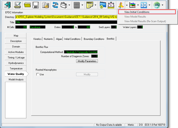
Figure 61 View Initial Conditions.
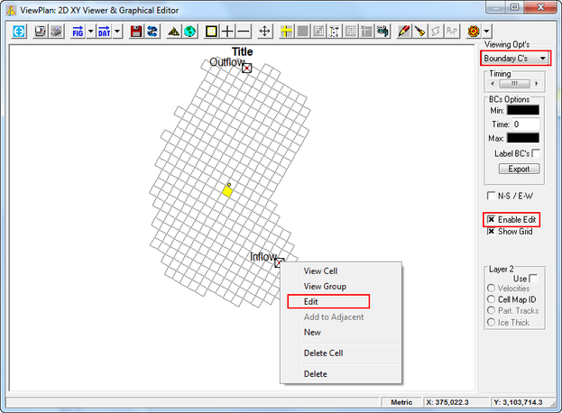
Figure 62 View Plan Boundary Conditions.
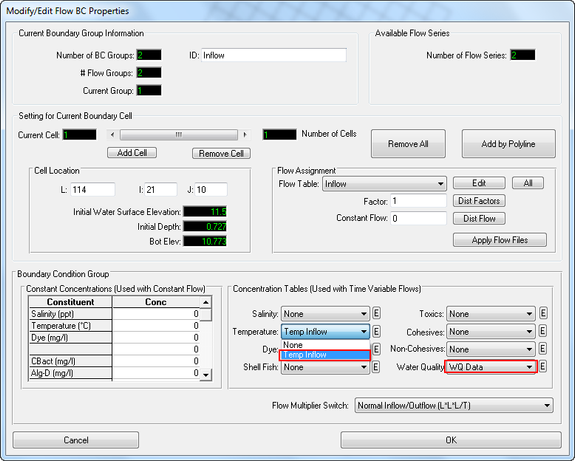
Figure 63 Modify/Set BC Properties: Inflow.
9. Click Save Project button in the main form, the Select Directory: Write Operation will now be displayed. Select Full Write in the Save Options frame; click Ok as shown in Figure 64.
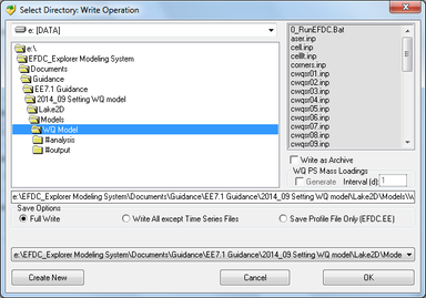
Figure 64 Apply Full write of the model.
4. Running the Model
1. Load the model
2. Select the Timing/Linkage tab and Model Run Timing
3. Set the Model start time to 0;
4. Set # of Reference Periods to 365;
5. Set Duration of reference periods to 24;
6. Set Time step to 100 Figure 65.
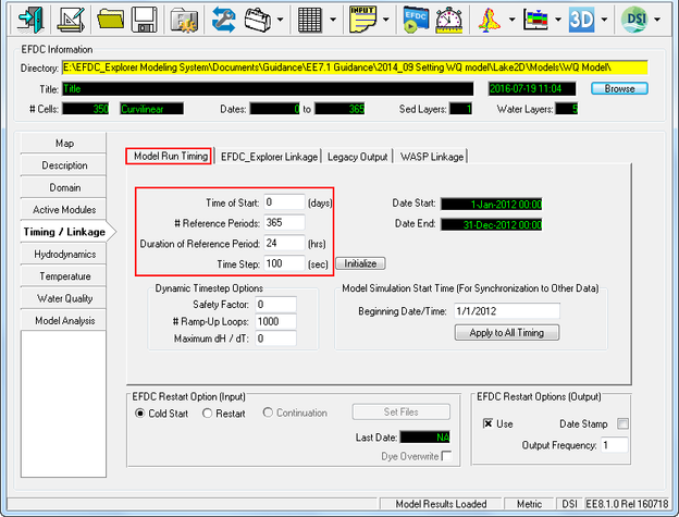
Figure 65 Main Form – Time / Linkage: Model Run Timing.
6. Navigate to the EFDC_Explorer Linkage tab and set the Linkage Output Frequency to 60 as shown in Figure 64.
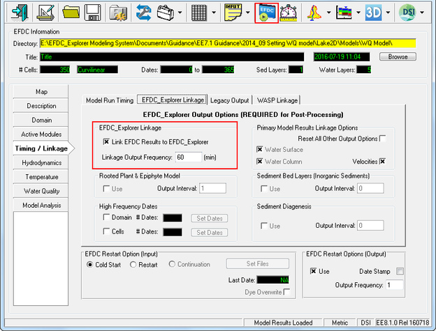
Figure 66 Main Form – Time / Linkage: EFDC_Explorer Linkage.
7. Check link EE to the EFDC_DSI model on the Main Form, click Settings button and browse to the EFDC_DSI model provided. The default location is: C:\Program Files (x86)\DSI\EFDC_Explorer8.1 as shown in Figure 67.
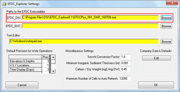
Figure 67 EFDC Executable file.
8. Click Run EDFC ![]() button on the Main Form; next enter number of OMP Threads then click Run EFDC+ button to run the model as shown in Figure 68.
button on the Main Form; next enter number of OMP Threads then click Run EFDC+ button to run the model as shown in Figure 68.
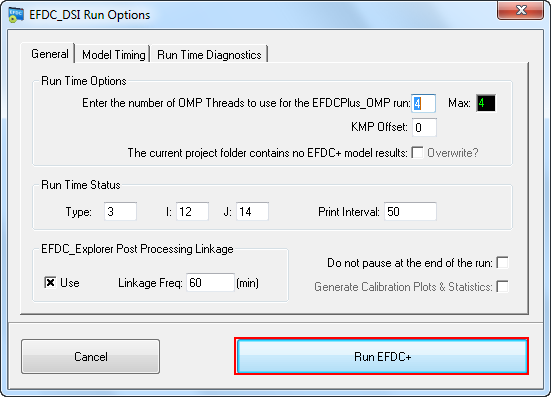
Figure 68 EFDC_DSI Run Options.
5. Viewing Water Quality in EFDC_Explorer
1. ViewPlan Mode
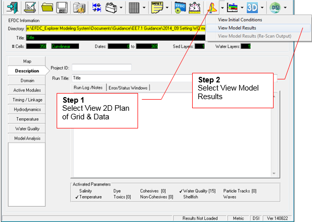
Figure 69 View Model results.
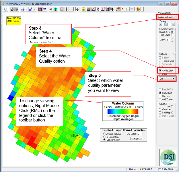
Figure 70 ViewPlan main form.
2. ViewProfile Mode
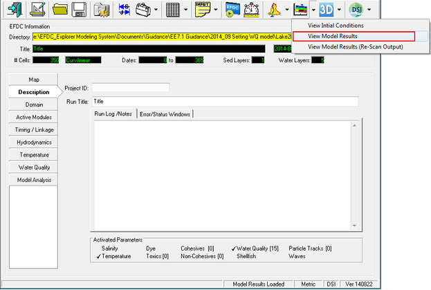
Figure 71 Vertical View Model results.
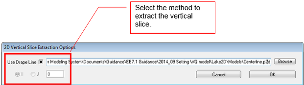
Figure 70 2D Vertical Slice Extraction Options.
The user can define a polyline by clicking Active Polyline Tools ![]() on 2D ViewPlan form to draw a polyline then RMC to end; next put a name for the polyline then save the polyline that can later used for slice/extraction as shown in Figure 73.
on 2D ViewPlan form to draw a polyline then RMC to end; next put a name for the polyline then save the polyline that can later used for slice/extraction as shown in Figure 73.
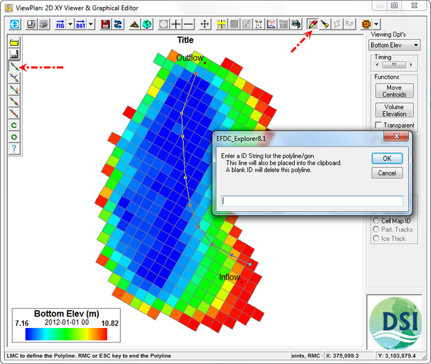
Figure 73 User Defined Profile/Slice Extraction Line Definition.

Figure 74 ViewProfile example showing salinity at one snapshot.
3. Vertical Profile Lines from ViewPlan Mode
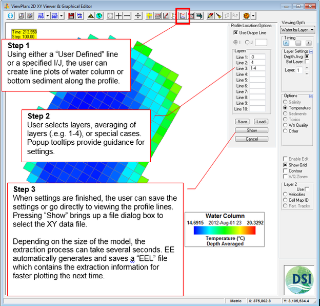
Figure 75 Longitudinal Profile tool.
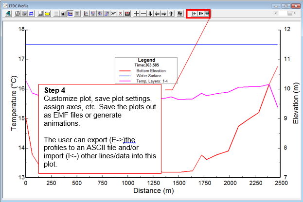
Figure 76 Water Column longitudinal profile of Temperature.