...
After finish import data series, go to Boundary Conditions tab, RMC on Inflow BC group under Flow sub-tab and select Edit Boundary Group to open the Flow Boundary Conditions form to link the concentration data to the boundary group. In this form, in the Time Varying Concentration tab under Boundary Group Condition frame, click on the drop-down menu of all concentration constituent and select the corresponding concentration data series to link them to the BC group as shown in Figure 23 below.
| Anchor | ||||
|---|---|---|---|---|
|

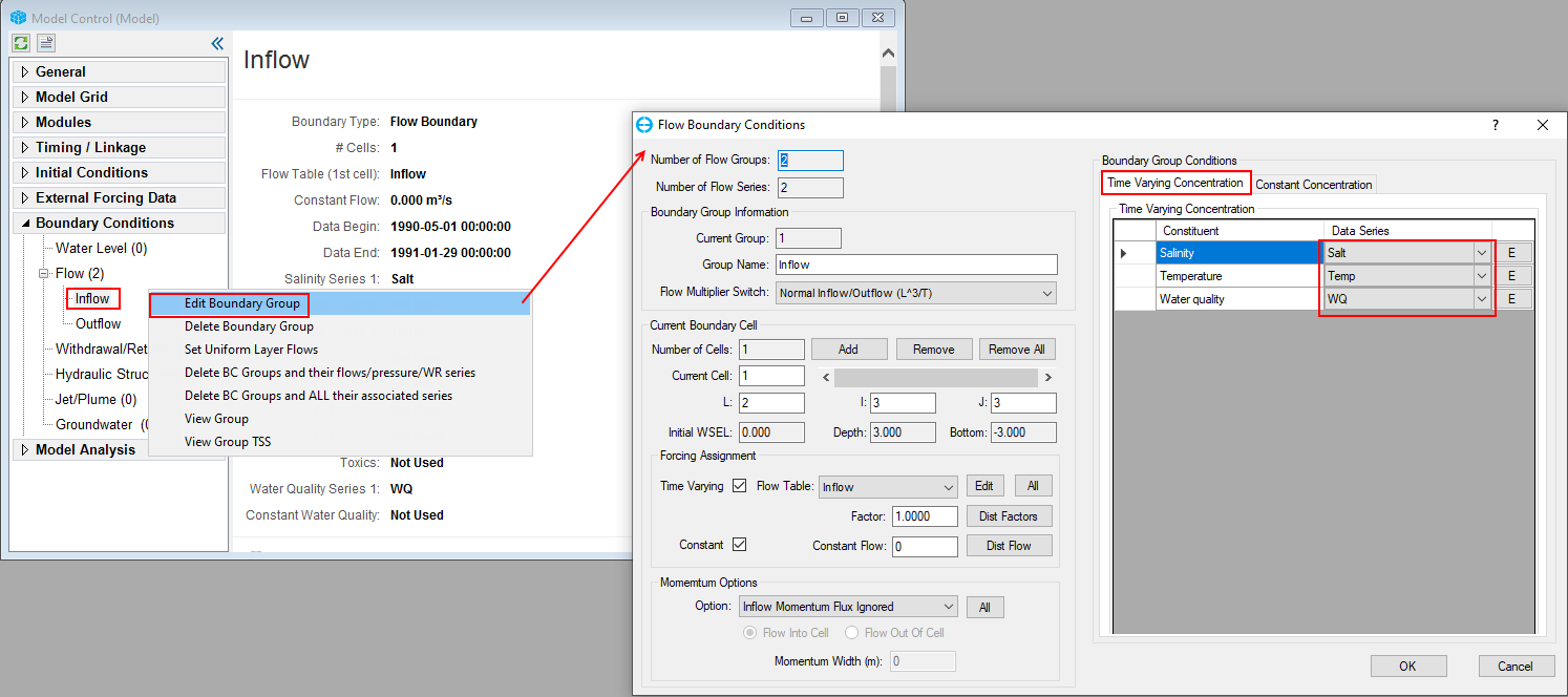
Figure 23. Link concentration data series to BC group.
...
From the Model Control form, RMC on Shellfish Farm module sub-tab under the Modules tab, then click on Settings option to open Shellfish Farm setting form as shown in 499679497 Figure 24 below.
| Anchor | ||||
|---|---|---|---|---|
|


Figure 2324. Shellfish Farm Settings (1).
...
- (1) type 1 in Number of Shellfish Species blank to add new shellfish farm species,
- (2) then click on Edit Species button to open Shellfish form to set species characteristics
- (3) Type in species name
- (4) Under Shellfish form, go to General tab, set parameters as shown in Figure 2425 below.
| Anchor | ||||
|---|---|---|---|---|
|

Figure 2425. Shellfish form – General tab.
Go to Infiltration tab, then set parameters as shown in Figure 2526 below.
| Anchor | ||||
|---|---|---|---|---|
|

Figure 2526. Shellfish form – Infiltration tab.
Go to Respiration tab, then set parameters as shown in Figure 26 below.
| Anchor | ||||
|---|---|---|---|---|
|

Figure 2627. Shellfish form – Respiration tab.
Go to Growth tab, then set parameters as shown in Figure 2728 below.
| Anchor | ||||
|---|---|---|---|---|
|

Figure 2728. Shellfish form – Growth tab.
Go to Mortality tab, then set parameters as shown in 499679497 Figure 29 below.
| Anchor | ||||
|---|---|---|---|---|
|

Figure 2829. Shellfish form – Mortality tab.
Go to Excretion tab and set parameters as shown in Figure 2930 below.
| Anchor | ||||
|---|---|---|---|---|
|

Figure 2930. Shellfish form – Excretion tab.
Go to Spawning tab and set parameters as shown in Figure 3031 below.
| Anchor | ||||
|---|---|---|---|---|
|

Figure 3031. Shellfish form – Spawning tab
After finish setting shellfish characteristics, click OK button to save settings and close form.
From Shellfish Farm form, go to Farm Settings tab as shown in Figure 3132 below. From this tab,
- (1) Type in 3 into Number of Farm Zone box to set 3 shellfish farm zones
- (2) Set shellfish farm zones parameters in Death Rate for each farm zone (group) in the Shellfish Farming Zones frame
| Anchor | ||||
|---|---|---|---|---|
|

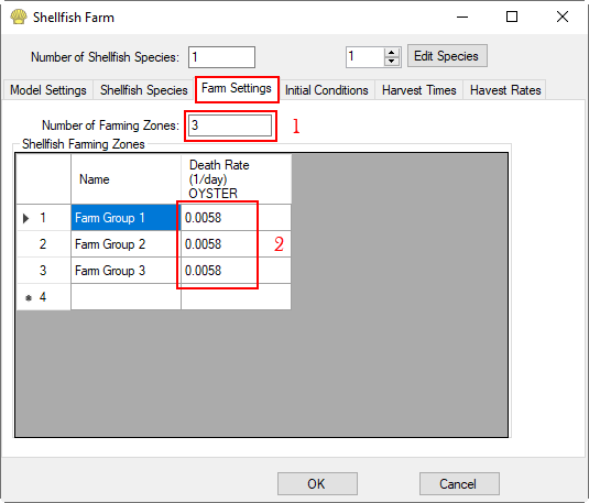
Figure 3132. Shellfish Farm – Farm Settings tab.
From Shellfish Farm form, go to Initial Conditions tab to assign the shell farm position and initial number of individual as shown in 499679497 Figure 33 below. From this tab, under Initial Individuals and Harvest Rateframe,
- L, J, J columns: cell index of the shellfish farm
- Zone: Farm zone index
- IC# Oyster: Initial number of individuals
| Anchor | ||||
|---|---|---|---|---|
|

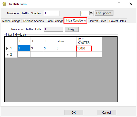
Figure 32 Shellfish 33 Shellfish Farm – Initial Conditions tab.
...
From the Model Control form, go to the Timing/Linkage tab | RMC on Timing sub-tab (Figure 3334). Set the Reference Date/Time to the base year of the study. Typically, this date is the 1st of some calendar year but this is not required, and any date/time is acceptable. Users can use the J<->G button to convert from the Julian calendar to the Gregorian calendar or vice-versa. In this exercise, the base date is 1990-01-01.
...
Growth Step is the minimum number of iterations for each time step before increasing DTDYN. Maximum Time Step is the maximum allowed time step in seconds. If this value is too high the model will crash. Users can refer to the EE Knowledge Base on Timing for more details.
Click on the OK button to save the settings and close form before moving forward to the next steps
| Anchor | ||||
|---|---|---|---|---|
|

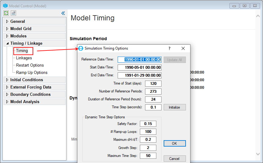
Figure 3334. Simulation Timing settings.
Returning to the Model Control form, expand the Timing/Linkage form, go to Linkage tab | RMC on EFDC_Linkages sub-tab (499679497Figure 35) to set the output frequency. In the EFDC Model Linkages form that pops up, select Link EFDC Results to EFDC_Explorer in the EFDC_Explorer Linkage tab and frame, and set the Linkage Output Frequency
In this exercise, set Linkage Output Frequency to 1440 minutes. This means EFDC will record the output every day for displaying.
Note: Smaller the output frequency, larger the output file size.
| Anchor | ||||
|---|---|---|---|---|
|
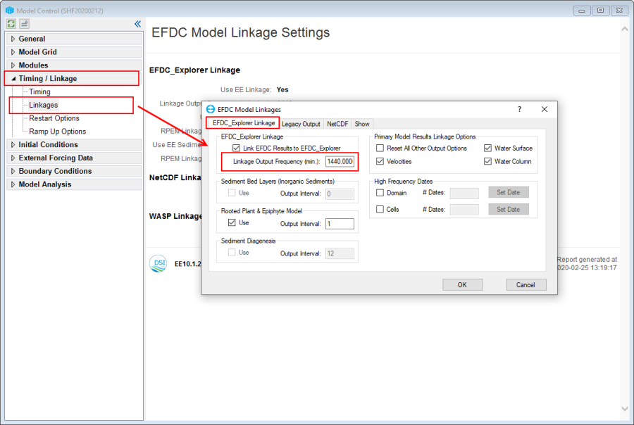
Figure 3435. EFDC_Explorer Linkage setting form.
Save the model and click on Run EFDC button to run the model. The EFDC+ Run Options form will appear. In EFDC+ Run Options form, set the Number of Threads to use for the EFDC+ run in Run Time Options # OMP Cores Used is 1 in case the demo license is using. Note that the number of threads cores use for EFDC+ run must be smaller than the total number of threads Available CPU Cores. (see Figure 36).
Set the KMP Offset to set the threads that will be passed over when running model. For example, if KMP Offset is set to 2, that means the thread used for EFDC+ run will start from the 3rd thread. This can be used if you are running multiple models on one machine, so the models run on different threads.
Note: If the model has existing results, please check on the Overwrite check box to run and save new results.
...
| Anchor | ||||
|---|---|---|---|---|
|
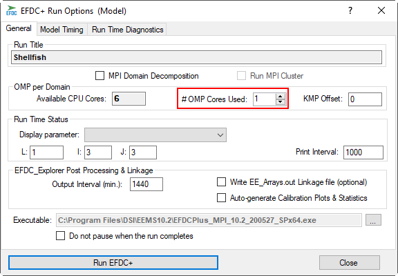
Figure 3536. EFDC+ Run Options form.
Click on Run EFDC+ button to start running model
...
(see Figure 37
| Anchor | ||||
|---|---|---|---|---|
|
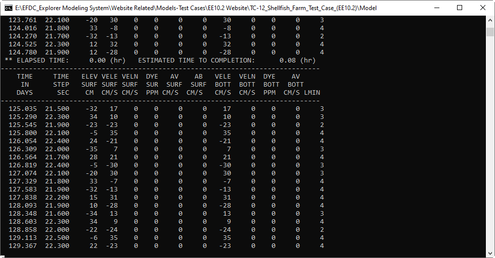
Figure 3637. EFDC+ run window.
Step-by-Step Guide for Model Output Visualization
...
After each simulation run finishes click on Refresh Output  button in the toolbar to refresh the model output.
...
From the 2DH View window, in the Layer Control form,
- (21) Click on the Add New Model Layer button to open 2DH View Option form which is used to select layer to add to 2DH View.
- (32) Select the parameter that users want to add to the 2DH View in Primary Groups (Shell Farm) and Parameters drop-down menus , in this case the selected parameter is Velocities(e.g. Shell Length).
- (43) Click on the Add button to a add layer to the 2DH View (Figure 3738).
| Anchor | ||||
|---|---|---|---|---|
|

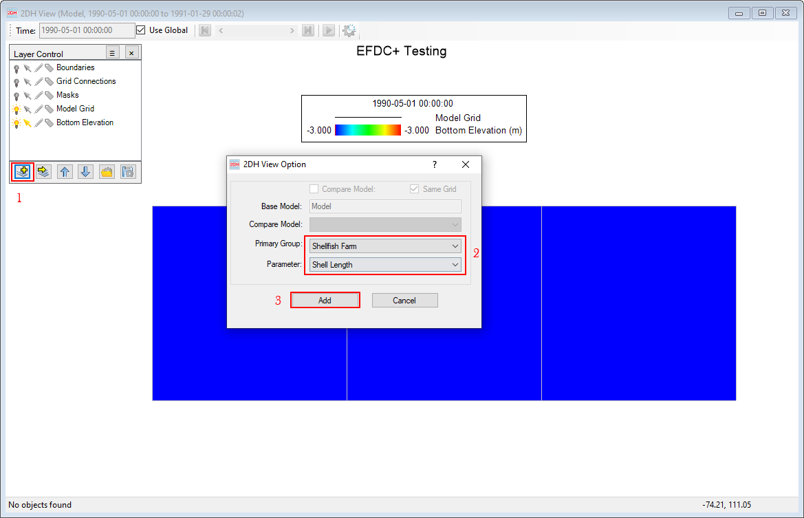
Figure 3738. Visualize model output in 2DH View (1).
- (5) RMC
- After the layer users want to modify the setting of the layer properties displayed on the legend

Figure 38. Edit layers in 2DH.
...
- Shell Length to the Layer Control, to see the change of this layer value the user follows steps below (see Figure 39):
- (1) Turn off the layer Bottom Elevation
- (2) Move the Timing Slide bar
- (3) See the value change on the legend or
- (4) Enable the selection arrow of the Shell Length layer
- (5) LMC on the cell then the output information of the selected cell at a specific time will be displayed on the yellow box (see Figure 40).
| Anchor | ||||
|---|---|---|---|---|
|
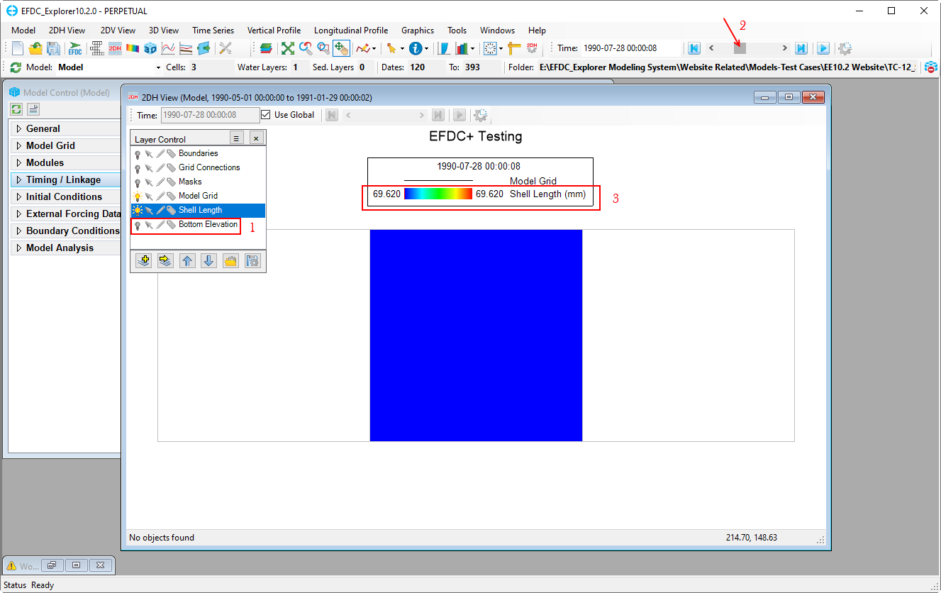
Figure 39. Visualize model output in 2DH View (2).
Anchor Figure 40 Figure 40
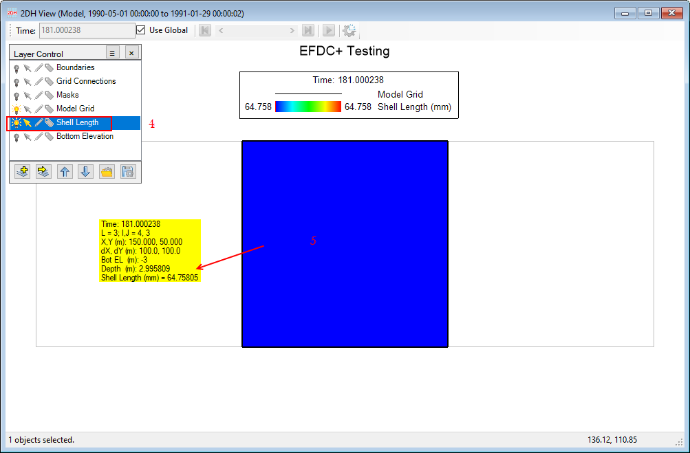
Figure 40. Visualize model output in 2DH View (3).
Model Verification
In this exercise, shellfish species characteristics are dry weight and shell length data series collected from the paper will be used to compare with the model output for verification. From EE interface, click on Time Series Plot icon in toolbars to open Extract Time Series Data form as shown in Figure 3941 below.
| Anchor | ||||
|---|---|---|---|---|
|

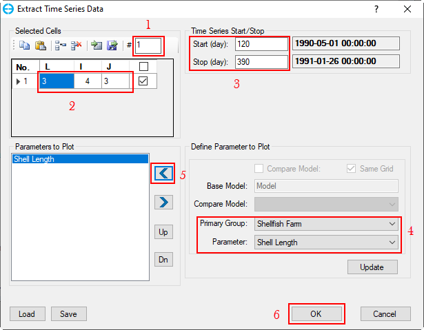
Figure 3941. Time Series Data Extraction.
...
- (1) Type in the number of cells that user want to plot to # blank , then (e.g. 1)
- (2) Then entering the L, I, and J index of each cell under Selected Cells frame. The user only needs to enter the L index, the IJ will be automatically updated.
- (23) The Time Series Start/Stop frame allows the user to set the time period of extracted data. As default this time period displayed as model simulation time period.
- (34) The Define Parameter to Plot frame allows the user to select parameters to plot in the same way as the Add Layer feature described for 2DH View. (refer to Figure 37). Note: If the user wants to modify an existing parameter or exchange it with another parameter, select that layer from the (5) Parameter to Plot frame and modify/change parameter settings, then click the Update button.After selecting a parameter from the (3) Define Parameter to Plot frame, (4) click e.g. Shell Length for Parameter)
- (5) Click the Left Arrow button to add a parameter; if the user wants to remove an already existing parameter, select that parameter in the (5) Parameter to Plot frame and click the Right Arrow button to remove. The Up and Down buttons are used to change the order of layers in the (5) Parameter to Plot frame.
- (5) The Parameters to Plot frame shows all parameters used for extracting.
- (8Note: If the user wants to modify an existing parameter or exchange it with another parameter, select that layer from the Parameter to Plot frame then click the Update button.
- (6) After finishing these settings, click the OK button to extract data. The time series data plot will be displayed as shown in Figure 4042.
| Anchor | ||||
|---|---|---|---|---|
|
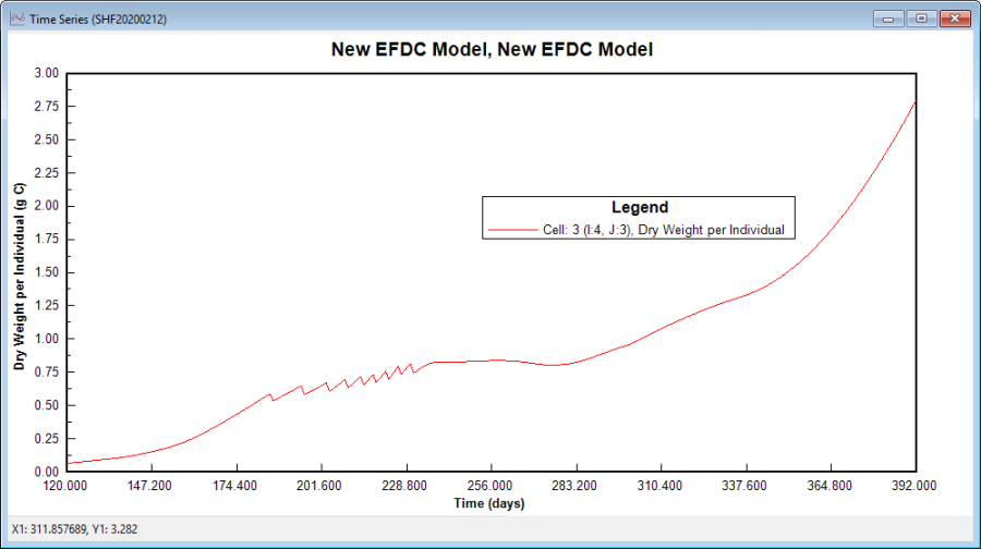
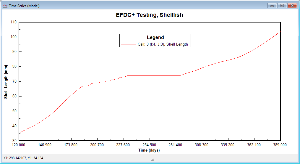
Figure 4042. Time series data plot: Shell Length.
From toolbar, click on Import Data Series icon, browse to data file name "Data_Dry weightShell Length.dat" in the Data folder, then click OK button to import data series as shown in Figure 41 belowseries as shown in Figure 43 below. The Enter the series index to import form pops up as shown in Figure 44, EE defines the model extracted time series is the first time series with index is 1 so the index of data time series imported will be consider as 2. In case if the users enters 1 so the model time series will be replaced with the data time series.
| Anchor | ||||
|---|---|---|---|---|
|

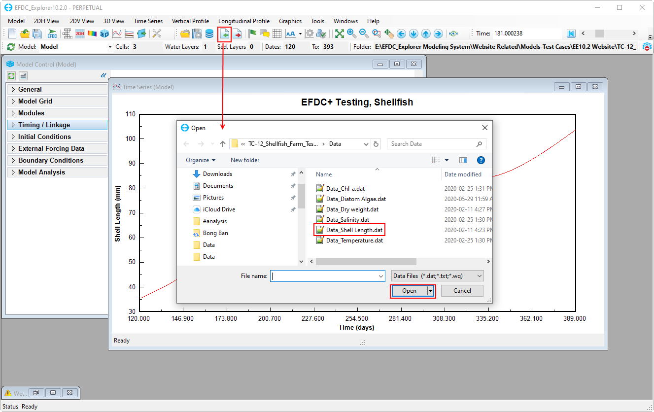
Figure 4143. Import external data series to existing plot.
Anchor Figure 44 Figure 44
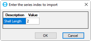
Figure 44. Enter the series index to import.
Anchor Figure 45 Figure 45
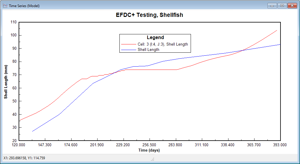
Figure 45. Modeled vs Data: Shell Length (1).
When the measured data is added, RMC on the legend to change the settings of data series for more clearly visualization of data series (the blue line) for more clearly visualization by RMC on the legend and change data series displayed as points as shown in Figure 4246 below.
| Anchor | ||||
|---|---|---|---|---|
|

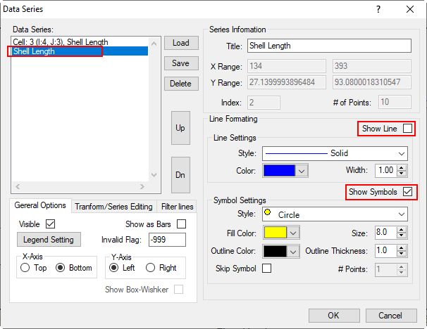
Figure 4246. Edit the data plot.
...
Anchor Figure 47 Figure 47
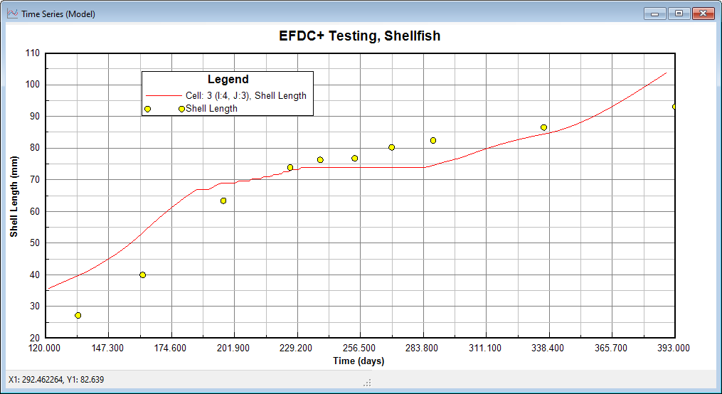
Figure 47. Modeled vs Data: Shell Length (2).
The user can also do the same steps as above to compare shell length dry weight data. The plot for shell length dry weight is shown in Figure 4348 below.
| Anchor | ||||
|---|---|---|---|---|
|

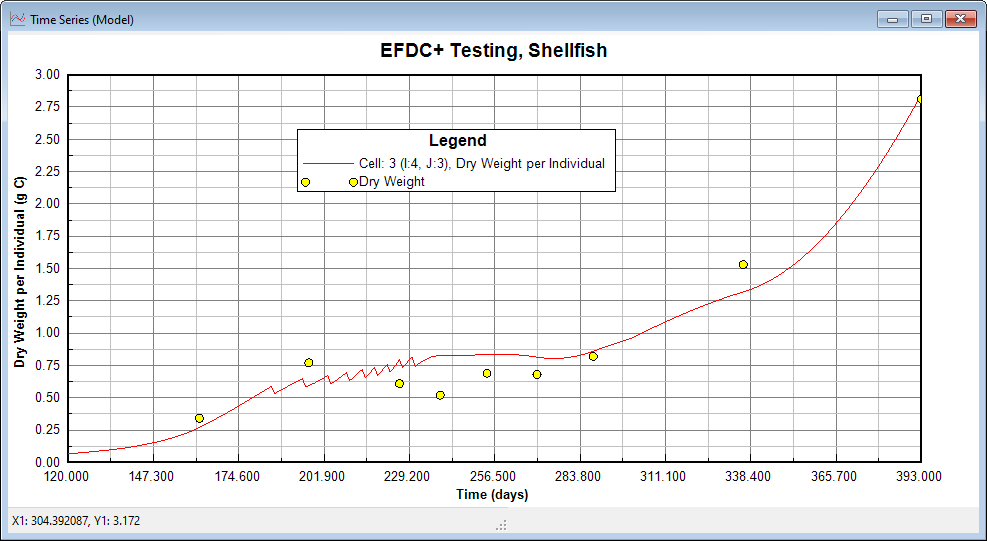
Figure 43. Time series comparison plot for shell length48. Modeled vs Data: Dry Weight.