This tutorial document is based on a steady-state problem from Thomann & Mueller (1987) “Principles of Surface Water Quality Modeling and Control” Sample Problem 6.10 (which was itself adapted from Driscoll et al., 1981).
...
- USGS gaging station upstream of WWTP
- Long term average summer flow = 100 cfs
- 7Q10 = 30 cfs (for min 7-consecutive day flow with a return period of once in 10 years)
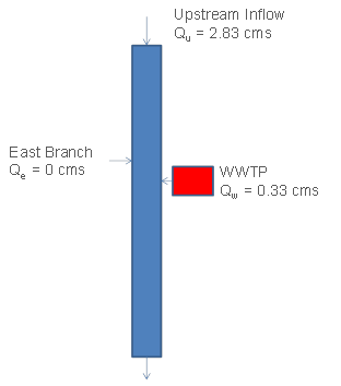
Figure 1. 1-D River schematic.
Velocity
- From the time of travel studies at various flows, U = 0.0513Q0.4; U (fps), Q (cfs)
...
2. From the empty main form shown in Figure 2 select the New Model button or press Ctrl + N from the keyboard.
| Anchor | ||||
|---|---|---|---|---|
|
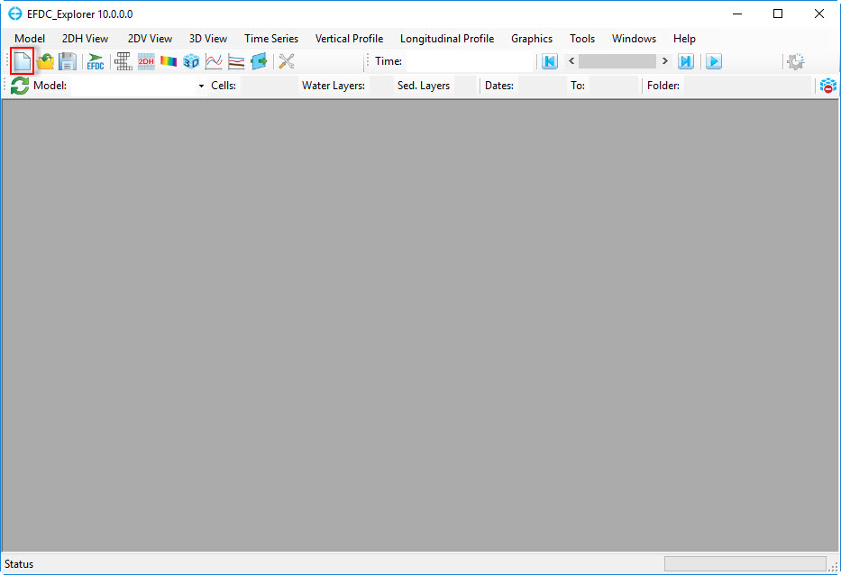
Figure 2. EFDC_Explorer main form.
The form is shown in Figure 3 should now be displayed.
| Anchor | ||||
|---|---|---|---|---|
|

Figure 3. Generate the EFDC model.
3. Select Generate Uniform Grid for this case
...
11. Press OK button, ignore the messenger box about UTM Zone as this is not in an actual physical location.
| Anchor | ||||
|---|---|---|---|---|
|
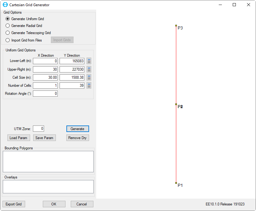
Figure 4. Generate EFDC model – with data.
12. In the Main Form, the General Information of the model is now displayed (Figure 5)
Anchor Figure 5 Figure 5
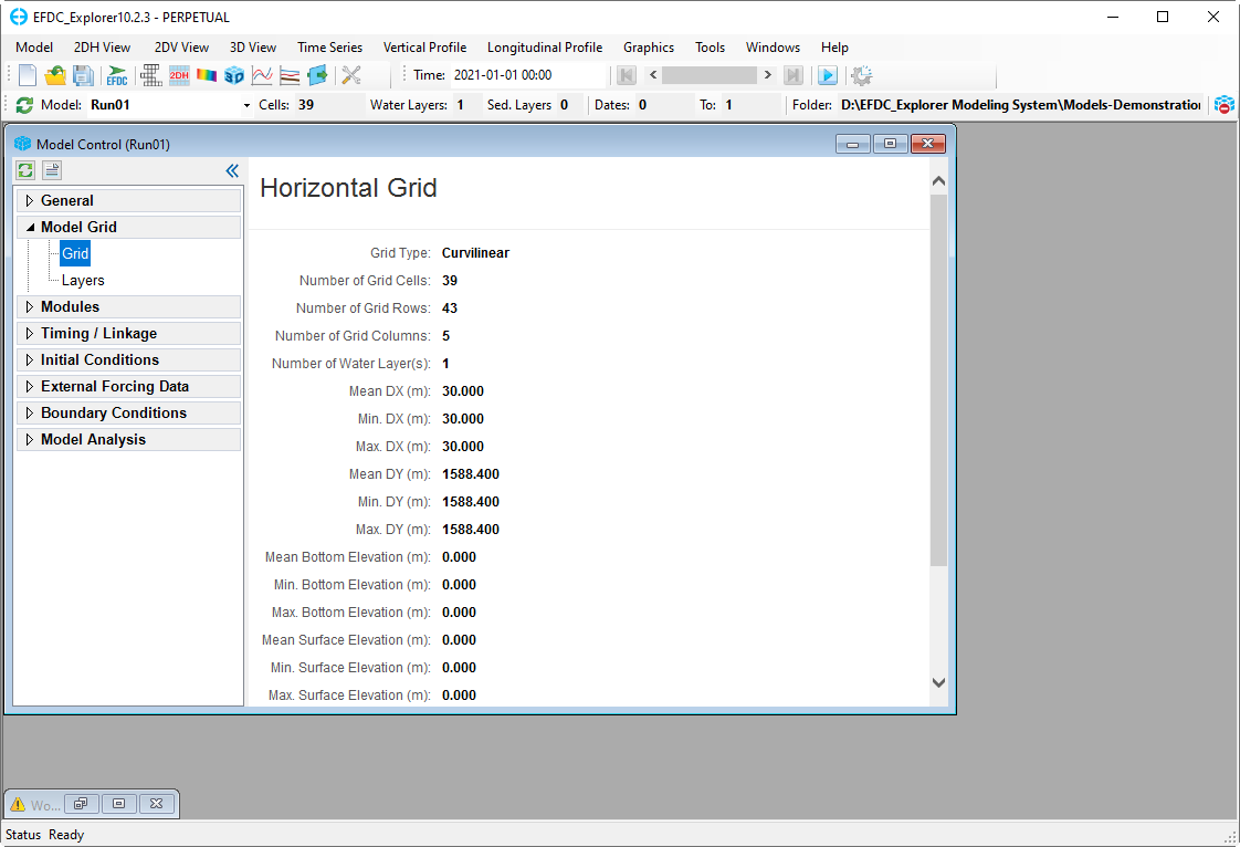
Figure 5. Model Control form – General tab.
3.1.2 Naming and Saving the Model
1. The user should enter the name of the project by RMC on Descriptions in General tab. These will become the default names in the View Plan and Time Series titles. Run ID, Run Title, Project Title as shown in Figure 6. The user also can keep track of changes from model to model by RMC on Change Logs and updating information in the form as shown in Figure 7.
Anchor Figure 6 Figure 6
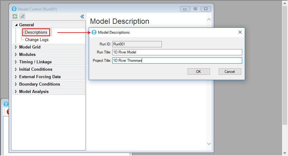
Figure 6. Model Description form – General tab.
Anchor Figure 7 Figure 7
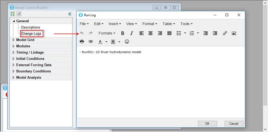
Figure 7. Change Logs form – General tab.
2. Save the model by selecting Save button from main menu toolbars and create a new directory and then, press OK button. (See Figure 8)
Anchor Figure 8 Figure 8
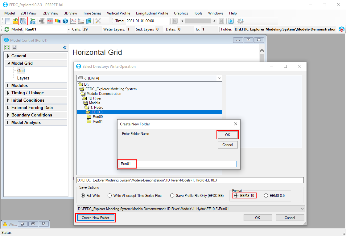
Figure 8. Saving the model.
3.1.3 Viewing and Checking the Grid
...
9. Click on any of the cells in the model domain to display an information box (yellow) that describes the cell L number, I and J number, the X, Y coordinates, bottom elevation, and depth.
| Anchor | ||||
|---|---|---|---|---|
|
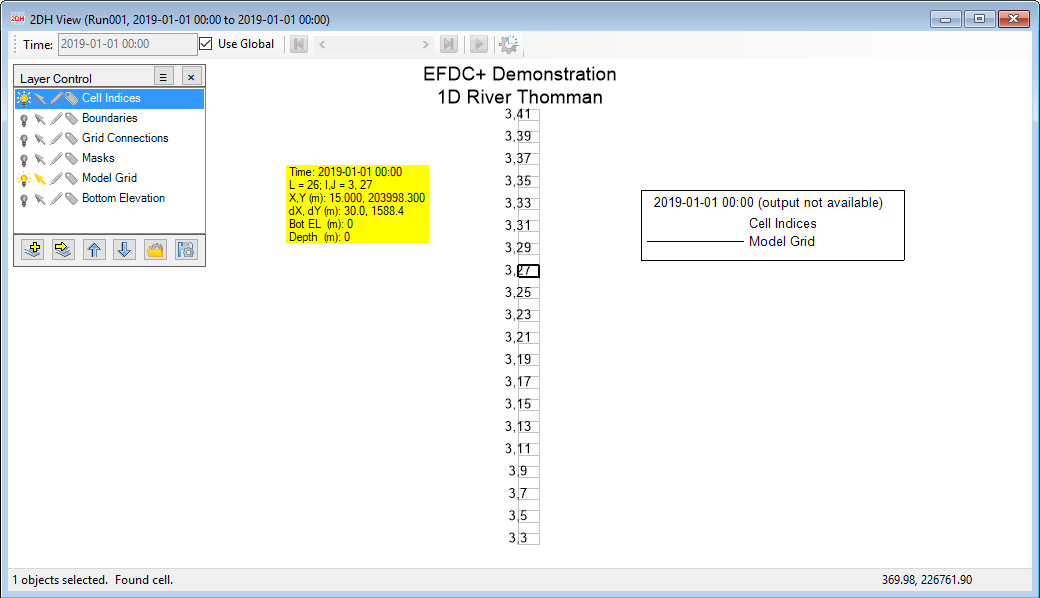
Figure 12 2DH View – cell indices.
3.2 Assigning Initial Conditions
...
3. In Assign Slope windows, set Start Value = 300 and J Slope = - 0.00005 then press OK. Note that this is a negative slope to assign from the DS to US end of the model, starting at 300 m at the DS end. (Figure 15). The model's bathymetry is updated and shown in Figure 15.1 after clicking on OK button on the Figure 15.
Anchor Figure 14 Figure 14
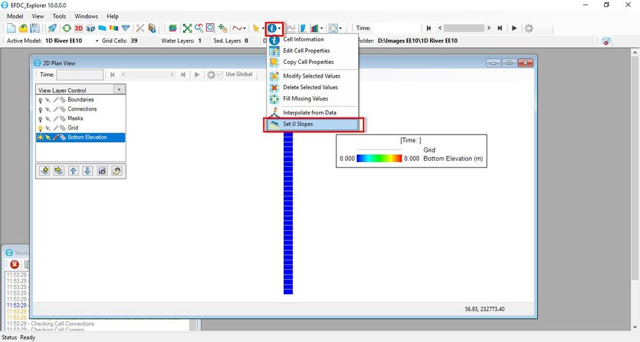
Figure 14. Open Assign Slope windows.
Anchor Figure 15 Figure 15

Figure 15. Assign data for model bathymetry.
Anchor Figure 15.1 Figure 15.1
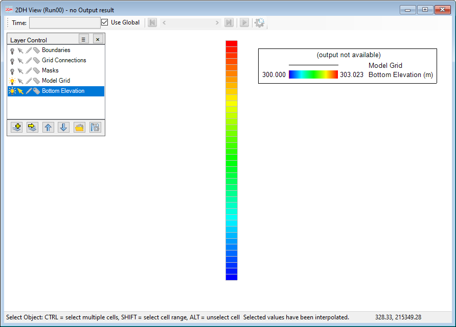
Figure 15.1 Model bathymetry after data Assignment.
3.2.2 Assigning Water Surface Elevation
...
Once the Model Bathymetry and Water surface elevation are assigned, we can check the data using the viewing options (2D plan view or the longitudinal profiles) by following the steps:
To check the data, return to the Main Form and select the Longitudinal Profile Plot button  The Data Extraction form is shown in Figure 18should now be in view. Using this form the user may select a profile along a pre-defined polyline (Drape file) or along an I or J entered by the user.
...
To add WSEL to the plot, in Primary Group choose Water level, in Parameter choose Water Surface Elevation then press Add to plot and OK button. This displays the plot shown inFigure 19.
| Anchor | ||||
|---|---|---|---|---|
|
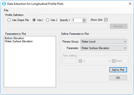
Figure 18. Data Extraction for Longitudinal Profile Plots.
...
Figure 22. Loading Label File.
Anchor Figure 23 Figure 23
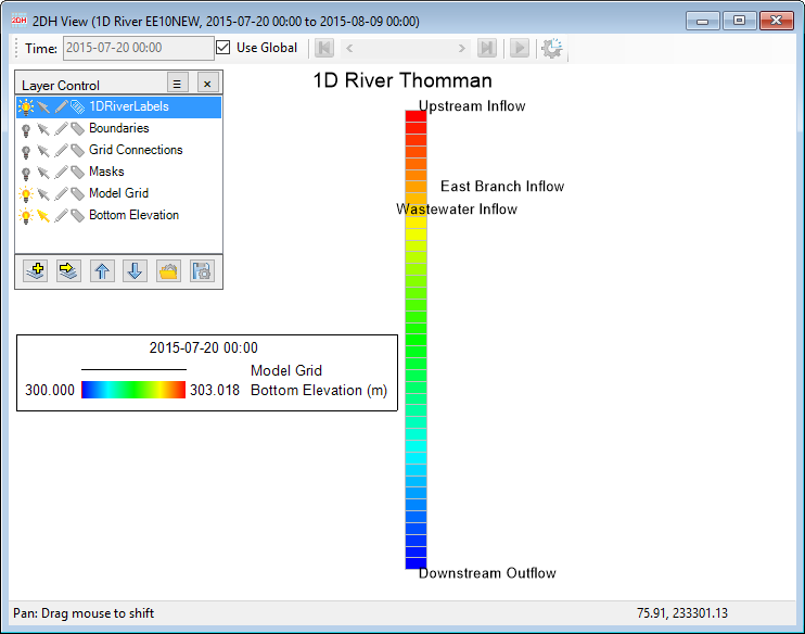
Figure 23. 2DH View: labels.
7. RMC on the label layer just loaded and select Properties to correctly align the labels and set the symbols as shown in Figure 24 and Figure 25.
...
8. Update the symbols and labels as desired such as shown in Figure 26.
| Anchor | ||||
|---|---|---|---|---|
|
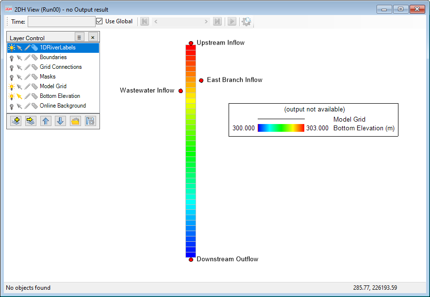
Figure 26. 2DH View with labels and makers.
9. Select Save
It is assumed for the purposes of this tutorial that three data recording stations are providing measured data. The user should create a file to record the locations of data recording stations called 1DRiverStations.dat (Figure 27)
...
Figure 28. Loading data posting file.
Anchor Figure 29 Figure 29
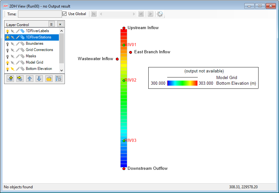
Figure 29. Overlay of data posting file on labels.
4 Boundary Conditions
The boundary conditions for this model have been taken from the Thomman textbook example and are summarized in the table below. In this case, dye is used as a proxy for the contaminant transport.
...
The Dye module will be added to the Modules, RMC on the Dye then select Settings, the form Dye Module will appear as shown in Figure 35.1 from this form, click on the drop-down list in the Type column then select Conservative Dye then click OK button.

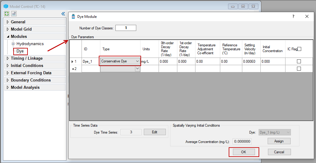
Figure 35.1 Dye Module – Conservative Dye setting.
...
Anchor Figure 39 Figure 39

Figure 39. 2DH View – Assign Boundary Conditions: Upstream
The Flow Boundary Conditions will now be displayed. This form is used to link the flow table to the BC.
...
All boundary conditions have now been set as shown in Figure 47.
Anchor Figure 43 Figure 43
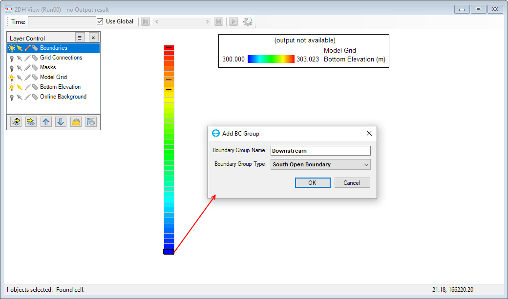
Figure 43. Downstream Boundary Conditions.
Anchor Figure 44 Figure 44
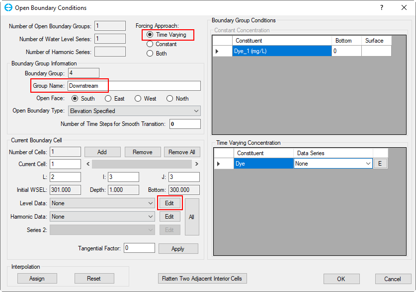
Figure 44. Set BC for Downstream.
...
- Select a cell (or multiple cells) first
- Click on the Time Series Plot button (
 ) from the main toolbar, the Extract Time Series Data form appears as shown in Figure 52, click OK button, a time series of the dye at those cells will be displayed as shown in Figure 53.
Anchor Figure 51 Figure 51
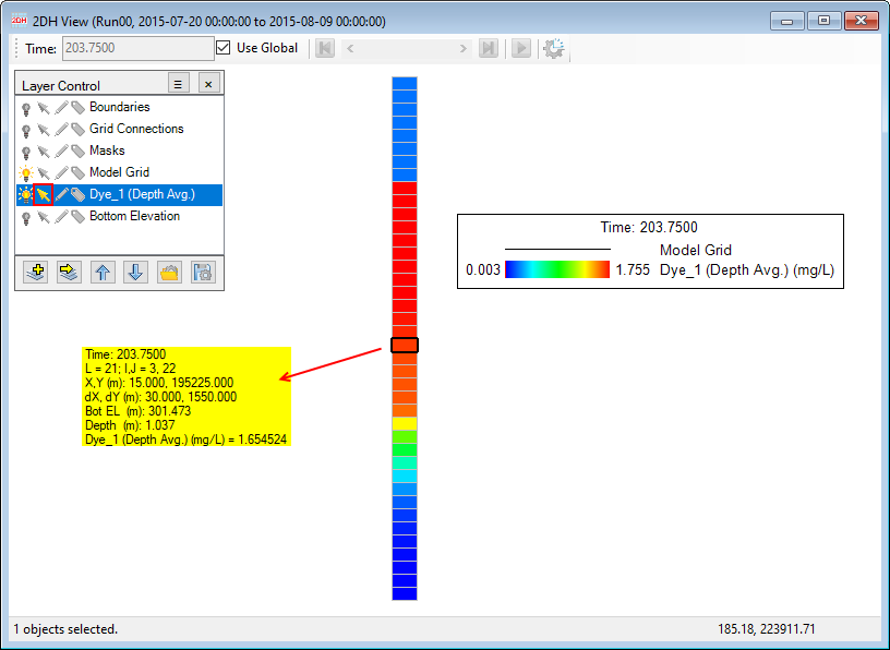
Figure 51. View dye concentration in the 2DH View.
Anchor Figure 52 Figure 52

Figure 52. View dye time series of selected cells (1).
Anchor Figure 53 Figure 53
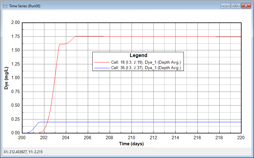
Figure 53. View dye time series of selected cells (2).
7 Model Result vs. Measured Data
...
- Click the Longitudinal Profile button (
 ) on the main toolbar, the Data Extraction for Longitudinal Profile form appears, select Use I option then enter 3 to Specify I.
 - Select Primary Group: Water Column, Parameter: Dye, Options: Depth Average for Layer Settings then click Arrow button to add to Parameters to Plots, then click OK button as shown in Figure 54.
- After click OK button, the plot will be displayed, use Ctrl+G to go to t=218 then click OK button as shown in Figure 55.
- In order to compare to measured data, load the data file by clicking the Import button (
 ) from main toolbar (data file name: DyeCX_T218_readMe.dat)
 - RMC on the legend to set the series line options for the data to dots using Line Formatting options as shown in Figure 56. As a result, the comparison plot is shown as Figure 57.
Anchor Figure 54 Figure 54

Figure 54. Define to plot longitudinal profile.
Anchor Figure 55 Figure 55
...