...
21 21 0 0 1 0 0 1 0
1 1 5 5.614220639170660E+05 3.697761609812420E+06
1 2 5 5.614094756223090E+05 3.697770022252650E+06
1 3 5 5.613951408251970E+05 3.697779601836410E+06
1 4 5 5.613811567605420E+05 3.697788947034500E+06
1 5 5 5.613674849040790E+05 3.697798083591720E+06
1 6 5 5.613543006637220E+05 3.697806894287380E+06
1 7 5 5.613410426823790E+05 3.697815754262280E+06
1 8 5 5.613279845603650E+05 3.697824480676230E+06
1 9 5 5.613151469448170E+05 3.697833059731270E+06
1 10 5 5.613025568625900E+05 3.697841473366020E+06
APPENDIX B
Mathematical Basis of CVLGrid
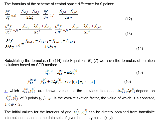
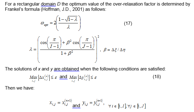
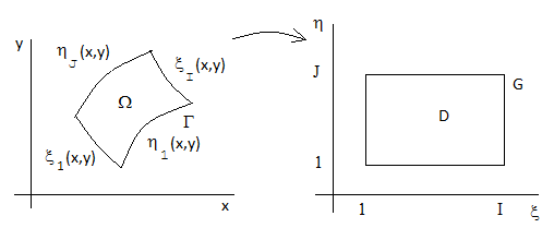
As mentioned previously, the Laplace equations are used by CVLGrid for grid generation. Therefore the family of orthogonal curves in a physical domain must be determined: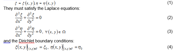
in which Ω is the physical domain with the closed boundary Г. Since this domain is not rectangular, the equations are converted into the logical domain D of the rectangle. The family of orthogonal curves must then be determined:
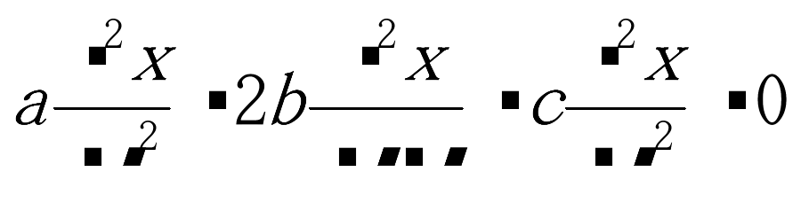
So that they satisfy the Laplace equations in the logical domain D: 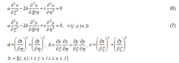
with the boundary conditions on four sides of rectangle D: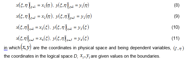
| Anchor | ||||
|---|---|---|---|---|
|