EE has filtering capabilities which are applicable for any time series plots. This involves the integration of a low pass and a high pass filtering to the time series plotting utility. Two type of filters (Lanczos and Fast Fourier Transforms) are available. This feature has also been added to the Time series Comparison form and Statistics tools in the Model Analysis tab as described in the next section.
The method of High- and Low-pass Filtering is that the instantaneous current velocity can be represented as the sum of time-averaged value and fluctuations of high and low frequencies as follows: vi=v+Vh+Vl (1)

where vi is instantaneous current velocity; v is time-averaged velocity; and Vh,Vl  are fluctuations due to the high and low frequencies respectively.
Based on the Fast Fourier Transform (FFT) method for energy spectra in frequency domain, these fluctuations were obtained dependent on the defined cut-off frequency i.e. at 1, 3, and 5 filtering hours. After that the inverse FFT was used to plot the high or low frequencies results.
High-Pass option: vi=v+Vh (2)
Low-Pass option: vi=v+Vl (3) 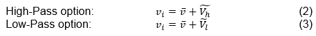
In the Time Series Plotting utility, the user can choose any time series to filter. There is an option to Create to new line in order to add this filtered line into the plot as shown in Figure 1. If Apply to this Line is selected the time series will be replaced with its filtered series, an example of which is shown in Figure 2.
| Anchor | ||||
|---|---|---|---|---|
|
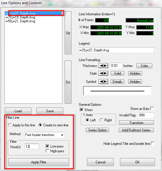
Figure 1 High and Low Pass Filter for Time Series Plotting.
| Anchor | ||||
|---|---|---|---|---|
|
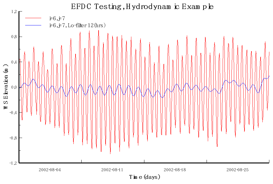
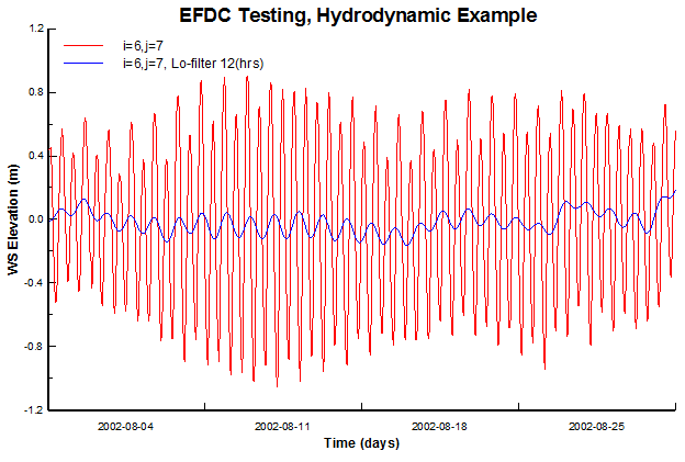
Figure 2 Time Series plot of WSEL (red) and low pass filter (blue) at location i=6, j=7.