...
Introduction
EFDC allows for multiple user defined sets of WQ sediment fluxes. This allows the user to change the fluxes seasonally, annually, or on whatever temporal basis the model needs. For each set/time block the user assigns a fixed flux for each constituent. The flux rates do not change during the time set for the block but can change from one time block to the next. The default is no time blocks, i.e. there is only one period that is constant. However, the user can configure as many time blocks as needed. This document shown the user how to specify the fluxes spatially and how to set the temporal changes of the fluxes.
Sometime when using this option the user is met with the warning: "WQBENMAP.INP Warning! Not all of the active cells assigned mud/sand". When specifying spatially varying benthic flux then the user must set a benthic flux map –warning tells you that if you haven't set the mapping for the various rates then you need to set it.
Description of
...
Hydrodynamic Model
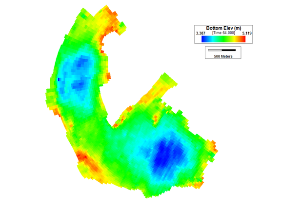
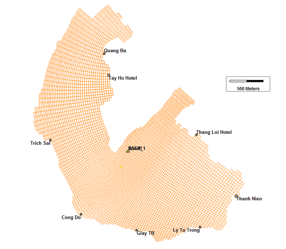
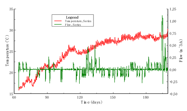
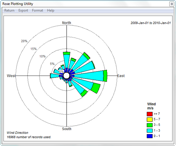
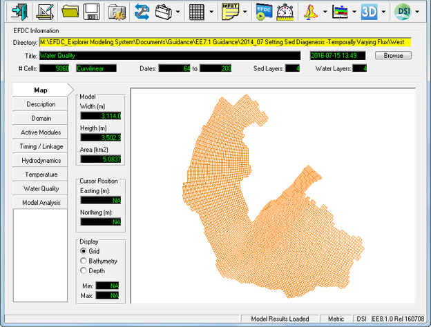
A hydrodynamic model of West Lake in Hanoi, Vietnam, has been built is available for download from the EE website. This model is used as the basis for building a water quality model that is part of this guidance document. Figure 1 provides a representation of the digital terrain model for West Lake. The locations of flow boundary conditions are presented in Figure 2. Flow discharge and temperature used for the model are shown in Figure 3 and a wind rose of the wind data used is shown in Figure 4.
...
...
...
Figure 1 EFDC model bathymetry in West Lake.
...
Figure 2 Boundary condition map in West Lake.
...
...
Figure 3 Flow boundary conditions.
...
...
Figure 4 Wind Rose of Wind Data.
...
...
Description of West Lake Water Quality Model
...
...
Figure 5 Open Water Quality model
...
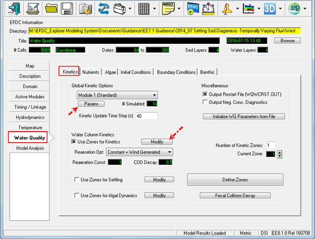
Water Quality – Kinetics Tab
The "WQ - Kinetics" tab is shown in Figure 6. Click the Params button display the list of parameters simulated in the West Lake model Figure 7.
...
...
...
Figure 6
...
Water Quality Tab: Kinetics.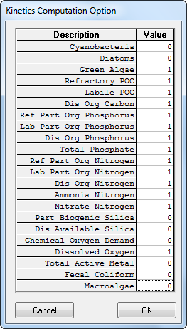
...
...
Figure 7 Kinetics Computation Option
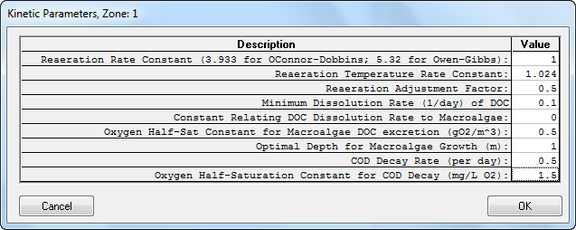
Click Modify button in the frame Water Column Kinetics to edit Parameter for current zone as shown in Figure 8.
...
...
...
Figure 8 Kinetics Parameters for zone.
...
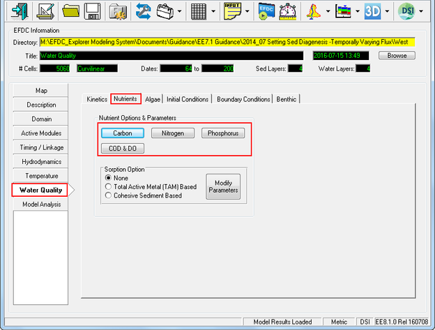
Water Quality – Nutrients
The WQ - Nutrients tab is shown in Figure 9. Within the Nutrient Options and Parameters frame, click Carbon button to edit the Carbon parameters; Nitrogen button to edit the Nitrogen parameters; Phosphorus button to edit the Phosphorus parameters, COD&DO button to edit the COD&DO parameters.
...
...
Figure 9 Water Quality Tab: Nutrients.
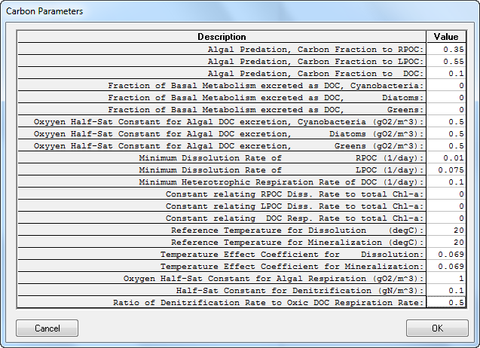
Figure 10 Nutrients: Carbon Parameters.
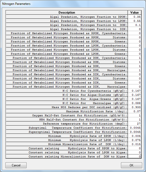
Figure 11 Nutrients: Nitrogen Parameters
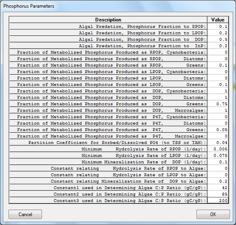
Figure 12 Nutrients: Phosphorus Parameters.
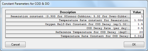
Figure 13 Nutrients: COD and DO Parameters.
...
...
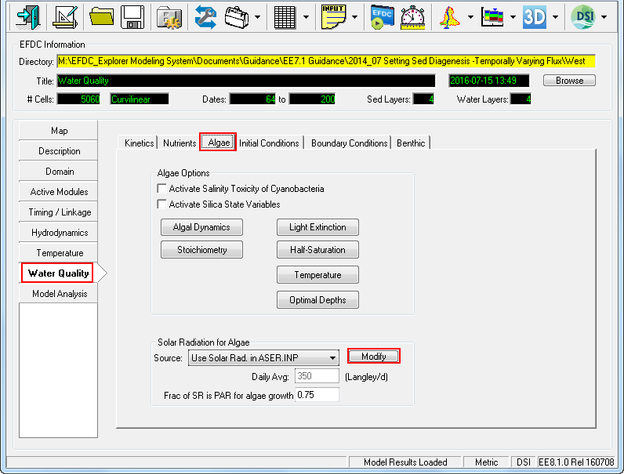
Water Quality – Algae
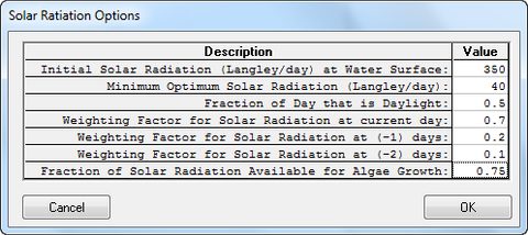
The WQ - Algae tab is shown in Figure 14; Within the Solar Radiation for Algae frame click Modify button to edit the Solar Radiation parameters shown in Figure 15.
...
Figure 14
...
Water Quality Tab: Algae.
...
Figure 15 Solar Radiation Options.
...
...
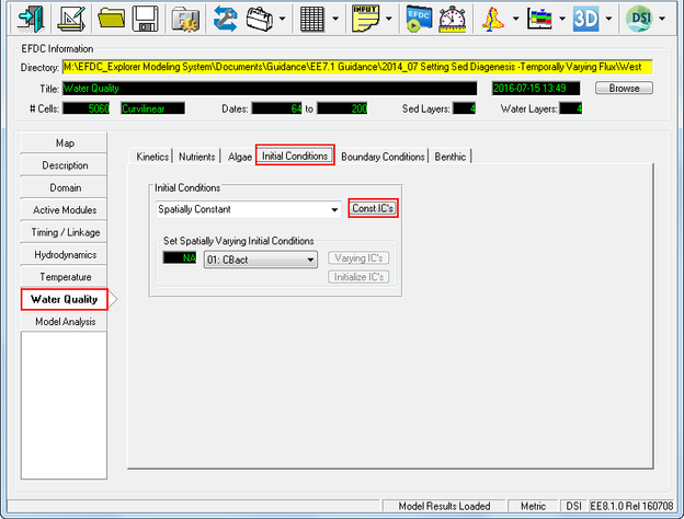
Water Quality – Initial Conditions
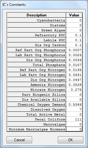
The WQ – Initial Conditions tab is shown in Figure 16. Within the Initial Conditions frame click Const IC's button to edit each of the water quality parameters Figure 17.
...
...
Figure 16 Water Quality Tab: Initial Conditions.
...
...
Figure 17 Initial Conditions Parameters.
...
...
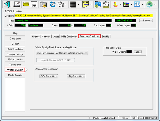
Water Quality – Boundary Conditions
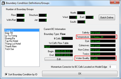
The WQ – Initial Conditions tab is shown in Figure 18; Use the same Time series data of Flow discharge; Temperature and Water Quality for eight boundaries are as shown in Figure 19.
...
...
...
Figure 18 Water Quality Tab: Boundary Conditions.
...
Figure 19 Boundary Conditions.
...
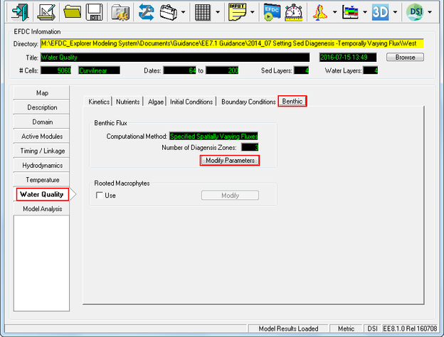
Sediment diagenesis for temporally varying fluxes
- Proceed to the Water Quality Tab Benthic sub tab shown in Figure 20
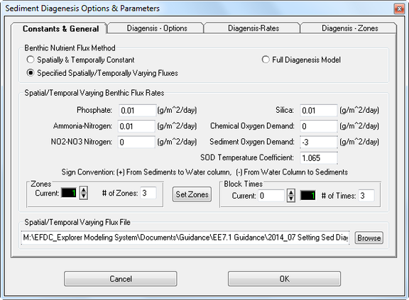
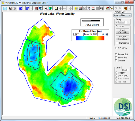
- Select the Modify Parameters button will now be displayed Sediment Diagenesis Option & Parameters as shown in Figure 21. The model domain is divided into three zones by three polygons as shown in Figure 22.
...
Figure 20 Water Quality Tab: Benthic.
...
...
...
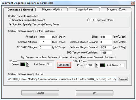
Figure 21 Sediment Diagenesis Option & Parameters.
...
...
Figure 22 Zones divided in the model domain.
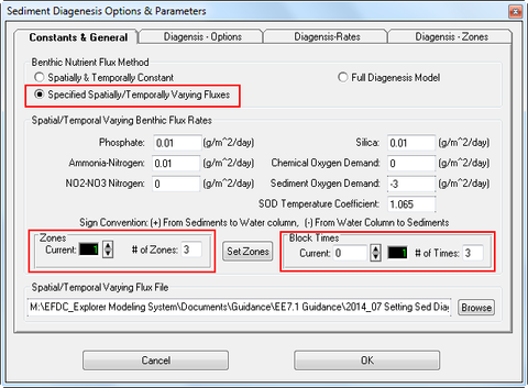
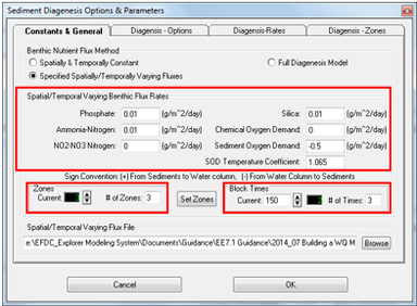
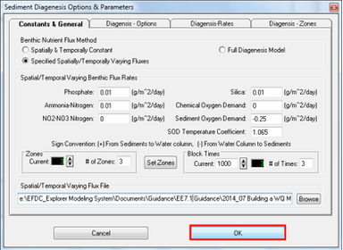
- From Sediment Diagenesis Option & Parameters form (Figure 21), in the top frame, Benthic Nutrient Flux Method select Specified Spatially/Temporally varying fluxes; Set the # Zone in the Zones box to 3; The # of time in the Block Times to 3 as shown in Figure 23
...
...
Figure 23 Set Zones and Block Times
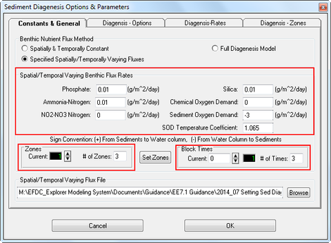
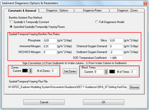
- Use the arrow buttons in the Zones and Block Times box to go to current zones and Block Time 1, set start time of current TIME BLOCK = 0; enter the values of parameters in the Spatial/Temporal Varying Benthic Fluxes Rates frame Figure 24.
...
...
...
Figure 24 Set parameter for Zones 1 and Block Times 1.
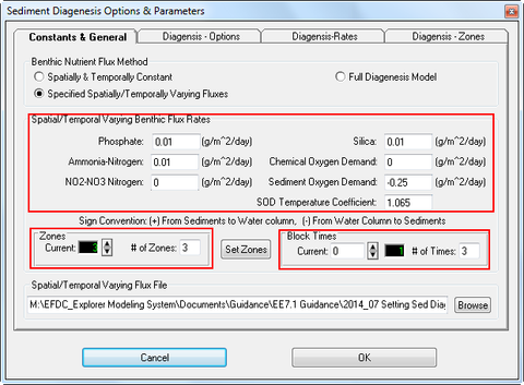
- Use the arrow buttons in the Zones box to go to current zones 2; enter the values of parameters in the Spatial/Temporal Varying Benthic Fluxes Rates frame as shown in Figure 25.
...
Figure 25 Set parameter for Zones 2 and Block Times 1.
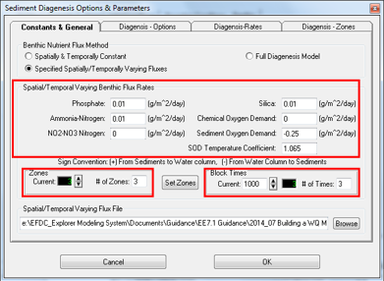
- Use the arrow buttons in the Zones box to go to current zones 3; enter the values of parameters in the Spatial/Temporal Varying Benthic Fluxes Rates frame as shown in Figure 26.
...
...
...
Figure 26 Set parameter for Zones 3 and Block Times 1.
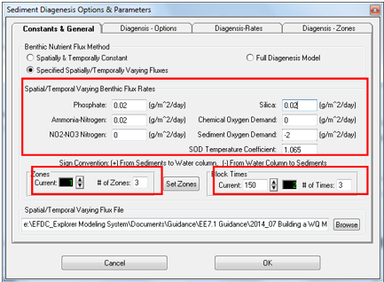
- Use the arrow buttons in the Zones box to go to current zones 1 and current Block Time 2, set start time of current TIME BLOCK = 150; enter the values of parameters in the Spatial/Temporal Varying Benthic Fluxes Rates frame Figure 27.
...
...
...
Figure 27 Set parameter for Zones 1 and Block Times 2.
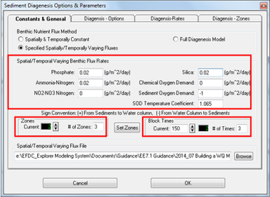
- Use the arrow buttons in the Zones box to go to current zones 2 and current Block Time 2; enter the values of parameters in the Spatial/Temporal Varying Benthic Fluxes Rates frame as shown in Figure 28.
...
Figure 28 Set parameter for Zones 2 and Block Times 2.
- Use the arrow buttons in the Zones box to go to current zones 3 and current Block Time 2; enter the values of parameters in the Spatial/Temporal Varying Benthic Fluxes Rates frame as shown in Figure 29.
...
...
Figure 29 Set parameter for Zones 3 and Block Times 2.
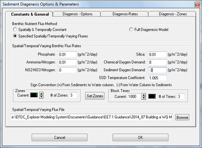
- Use the arrow buttons in the Zones box to go to current zones 1 and current Block Time 3, set start time of current TIME BLOCK = 150; enter the values of parameters in the Spatial/Temporal Varying Benthic Fluxes Rates frame as shown in Figure 30.
...
...
...
Figure 30 Set parameter for Zones 1 and Block Times 3.
- Use the arrow buttons in the Zones box to go to current zones 2 and current Block Time 3; enter the values of parameters in the Spatial/Temporal Varying Benthic Fluxes Rates frame as shown in Figure 31.
...
Figure 31 Set parameter for Zones 2 and Block Times 3.
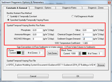
- Use the arrow buttons in the Zones box to go to current zones 3 and current Block Time 3; enter the values of parameters in the Spatial/Temporal Varying Benthic Fluxes Rates frame as shown in Figure 32.
...
...
Figure 32 Set parameter for Zones 3 and Block Times 3.
- Click Ok button to Return for the Main Form shown Figure 20 then Select the modify Parameters button after that select Setzones buttons to set zones Figure 33. When pressed, the form shown in Figure 34 is displayed.
...
...
Figure 33 Set parameter for Zones.
...
...
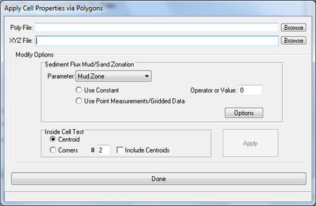
Figure 34 Sediment Diagenesis: Setting the initial conditions.
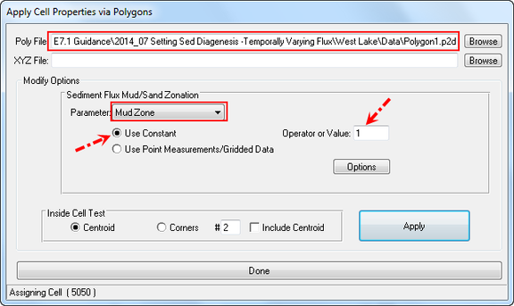
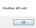
- From the Poly File box form browse to the Polygon file 1; select Mud Zone from the Parameter drop down; Select Use Constant and set the Operator or value = 1 as shown in Figure 35. Select Apply modified and message box will be displayed as shown in Figure 36, click OK button to apply value of Mud Zone 1.
...
...
...
Figure 35 Set Mud Zone for polygon 1.
...
Figure 36 Modified message box for Mud Zone 1.
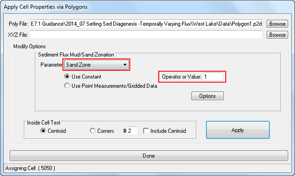
- Select Sand Zone from the Parameter drop down; Select Apply as shown in Figure 37, click ok to apply value of Sand Zone 1 as shown in Figure 38.
...
...
Figure 37 Sand Mud Zone for Zone 1.
...
...
...
Figure 38 Modified message box for Sand Zone 1.
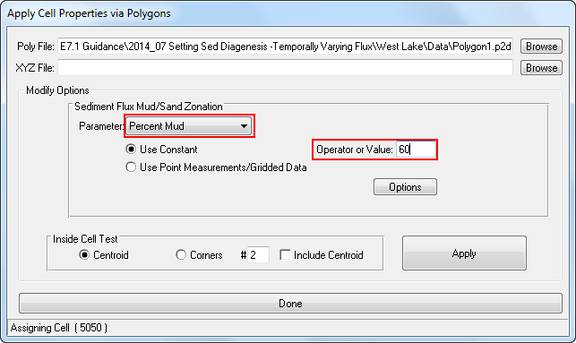
- Select Percent Mud from the Parameter drop down, set the Operator or value = 60; Select Apply as shown in Figure 39 , click ok to apply value of Percent Mud as shown in Figure 40.
...
...
...
Figure 39 Percent Mud for Zone 1.
...

Figure 40 Modified message box for Sand Zone 1.
- From the Poly File box form browse to the Polygon file 2 , do the same sub step from 14 to 16 for Zone 2 with: Mud Zone = 2, Sand Zone = 2, Percent Mud = 45
- From the Poly File box form browse to the Polygon file 2 , do the same sub step from 14 to 16 for Zone 2 with: Mud Zone = 3, Sand Zone = 3, Percent Mud = 30
- Click Done to apply these changes as shown in Figure 41, select ok as shown in Figure 42. Return to the Main Form shown in Figure 20.
...
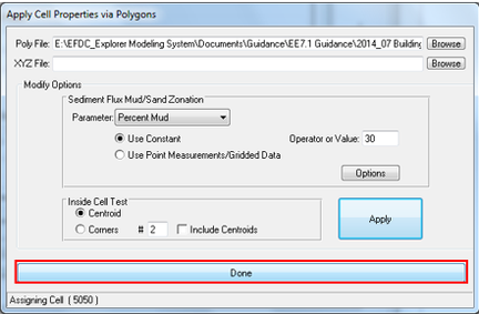
Figure 41 Done to apply these changes.
...
...
...
Figure 42 Select OK to apply all of changed parameters.
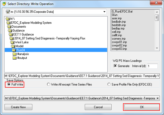
- Click Save Project button in the main form; The Select Directory: Write Operaton will now be displayed. Select Full Write in the Save Options frame, click Ok as shown in Figure 43.
...
...
...
Figure 43 Apply Full write of the model.
...
Viewing Sediment Flux in EFDC_Explorer
When the model has finished saving, open ViewPlan model.
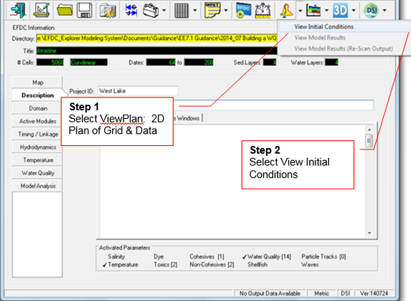
Figure 44 View Initial Conditions.
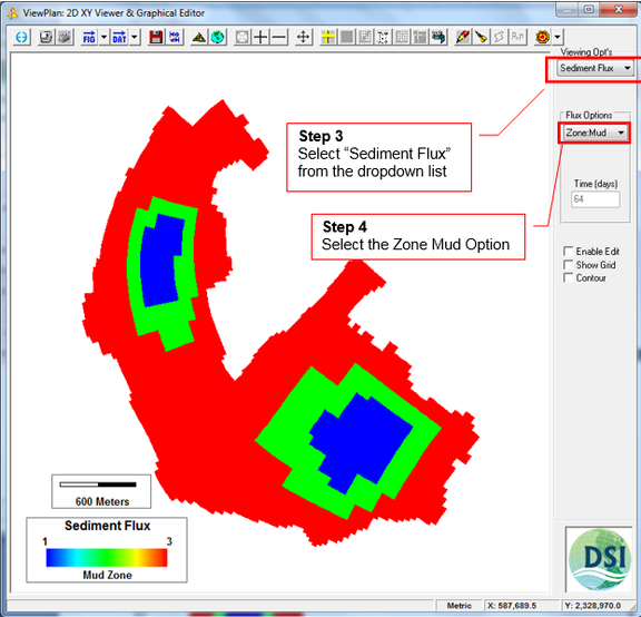
Figure 45 View Zone Mud.
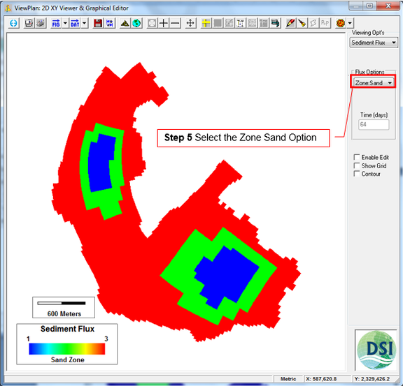
Figure 46 View Zone Sand.
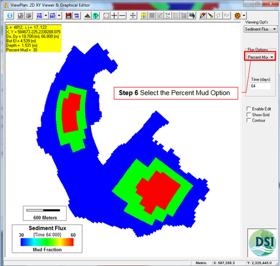
Figure 47 View Percent Mud.
...
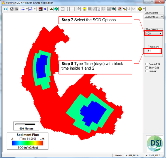
Figure 48 View Zone SOD with block time inside 1 and 2.
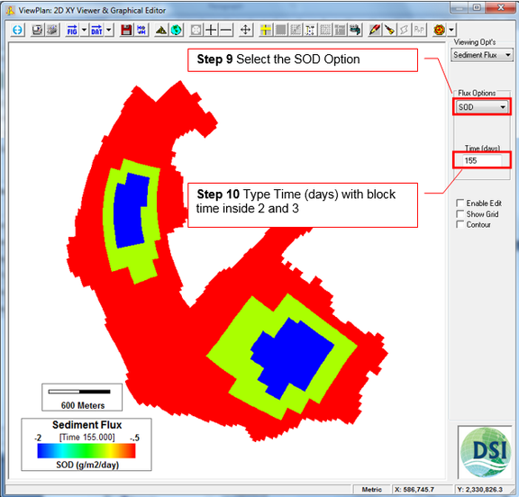
Figure 49 View Zone SOD with block time inside 2 and 3.
Note that if the option use the "Spatially & Temporally constant benthic flux" is selected then the SOD of zone displayed in ViewPlan is the same as that set by the user.
However, if the option "Specified spatially/Temporally varying fluxes" has been selected as described in this tutorial, then the SOD value of in ViewPlan will be different. This is due to the impact of percentage of mud specified by the user. This different depends on the equation for SOD:
SOD(time1) = xMud * sod(zone1,time1) + (1 - xMud) * sod(zone2,time1)
Where xMud = percent Mud /100
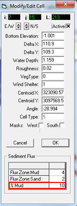
Figure 50 Setting Percentage Mud.