...
Lake Thonotosassa is the largest natural freshwater lake in Hillsborough County covering an
area of 849 acres (3.44 km2) (Hillsborough County Water Atlas). The lake is fed by Baker Creek
at the southeastern end of the lake and water flows out through Flint Creek on the northeastern
end to the Hillsborough River (Figure 1).
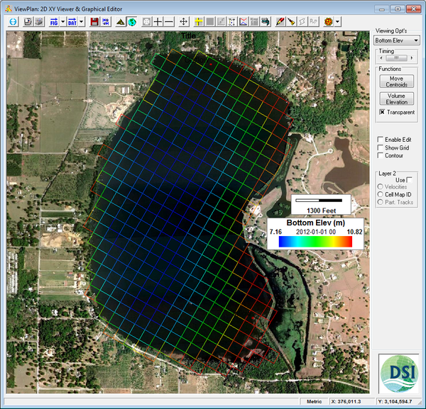
Figure 1 Lake Thonotosassa location map.
...
Open the Hydrodynamic model ( introduced in Build a 2D Lake Model (Level 1 Step-by-Step Guidance)) then add Winds wind data in the model as shown in Figure 6.
...
In the Main Form of EE, select Active Modules tab and Turn turn on the "Temperature and Water Quality" computations module as shown in Figure 9.
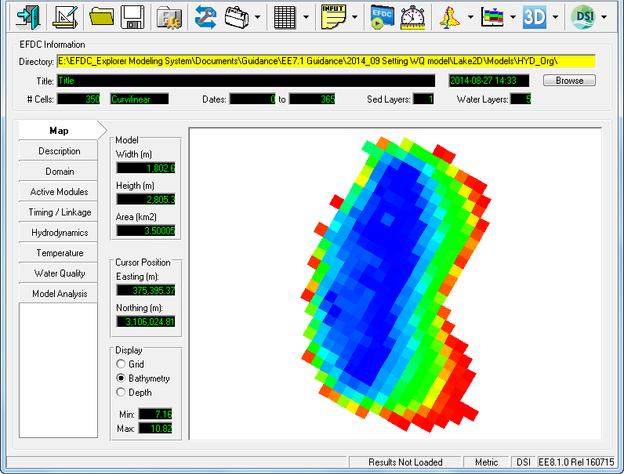
Figure 8 Open Hydrodynamic model.
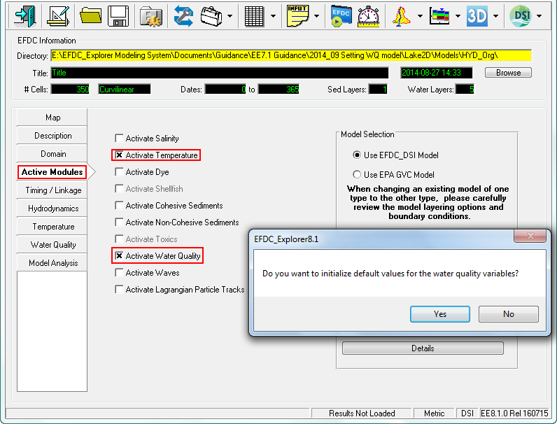
Figure 9 Activate Temperature and Water Quality.
Right after After the check box of for Activate Water Quality is enableenabled, the a prompt from EE will appear to ask if we want to initialize default values for the WQ variables as shown in Figure 10.
| Info |
|---|
Note that from EE7.3 and later we have the efdc.mdb file, which contains the default values for WQ. This saves the user a lot of time in manually entering as they no longer need to manually enter these values. If they say "No" they have to manually enter the values or import them from a previous model. |
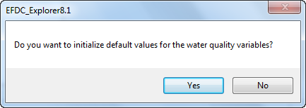
Figure 10 Yes/No to Initialize default values for WQ variables.
3.1 Create the
...
temperature boundary time series; the
...
atmospheric boundary time series and set IC for temperature
1. Proceed to the Temperature tab shown in Figure 11. From this form we can create the Temperature temperature boundary time series and the Atmosphere atmospheric boundary time series
2. Select the I for Edit button on Temperature for the Time series Data. This will display the form shown in Figure 12
3. Set the number of flow series to 1; Current current series 1
4. Set the title to "Temp Inflow" and type or copy and paste into the form for the time and Temperature temperature data (Figure 13)
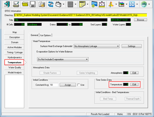
Figure 11 Main Form – Temperature Settings.
...
5. Return for the Main Form shown in Figure 9 and select the E button for Atmosphere Atmospheric
6. Repeat the above process for Atmosphere atmospheric data as shown in Figure 14
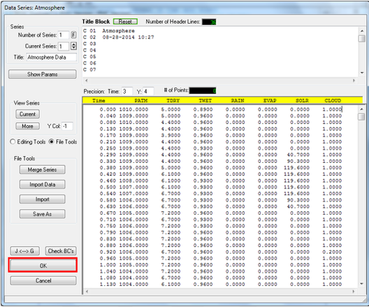
Figure 14 Boundary Condition: Atmosphere Atmospheric data.
7. Click OK button to return for the Main Form shown in Figure 11. In the Heat/Temperature frame LMC to Surface Heat Exchange Submodel box, the drop down list provides several options, including atmospheric Atmospheric linkage, Full Heat Balance, External Equilibrium Temperature, Constant Equilibrium Temperature and Equilibrium temperature (CE-QUAL-W2 method, EFDC_DSI only). Select Equilibrium Temp (CE-QUAL-W2 method) as shown in Figure 15.
8. In the Main Form shown Figure 9 11 then select the Settings button in the Heat/Temperature frame. When pressed, the form shown in Figure 16 is displayed, type Atmospheric Parameters from keyboard in the atmospheric parameters into the Value column then click Ok button.
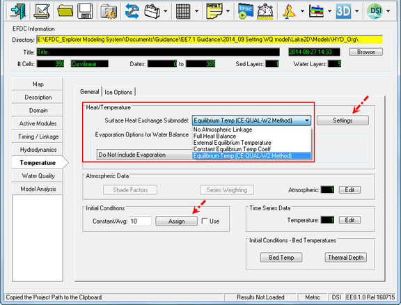
Figure 15 Select type of Surface Heat Exchange Submodel.
...
9. Select the Assign button for Temperature temperature to displays display the form shown in Figure 17
...
2. Click the Params button display the list of parameters simulated; type 1 for parameter simulated and 0 for not in the Lake Thonotosassa model simulated as shown in Figure 20.
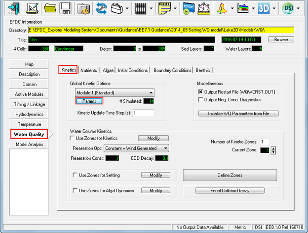
Figure 19 Water Quality Tab: Kinetics.
...
4. Click Modify button in the frame Water Column Kinetics | Use Zones for Algal Dynamics to edit Parameter for current zone as shown in Figure 24 22.
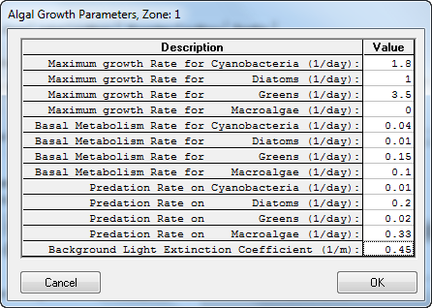
Figure 22 Algal Growth Parameters.
...
3.2.3 Water Quality – Algae
Proceed to the The "The WQ - Algae" tab; The WQ - Algae tab is shown in Figure 30; Within the Solar Radiation for Algae frame click Modify button to edit the Solar Radiation solar radiation parameters shown in Figure 31.
...
3.2.4 Water Quality – Initial Conditions
Proceed to the The "The WQ – Initial Conditions" tab; The "WQ – Initial Conditions" tab is shown in Figure 32. Within the "Initial Conditions" frame click Const IC's button to edit each of the water quality parameters Figure 33.
...
3.2.5 Water Quality – Boundary Conditions
1. Proceed to the The "The WQ – Boundary Conditions" tab; The "WQ – Initial Conditions" tab is shown in Figure 34; Click Edit button in the Time series Data frame. This will display the form shown in Figure 35.
...
2. Set the number of series to 1; Use the arrow buttons below to go to series 1. Set the title to "WQ Data" and type or copy and paste into the form for the time and Cyanobacteria data Figure as shown in figure 36 .
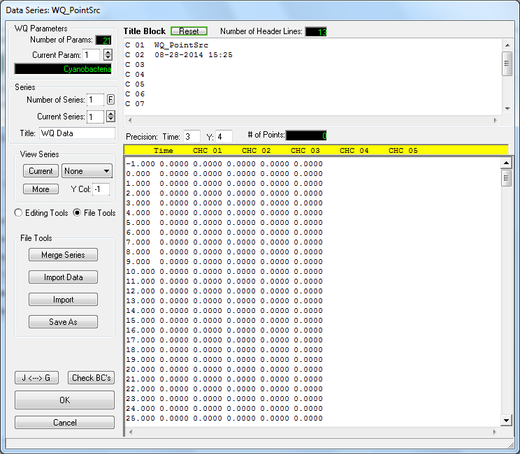
Figure 36 Boundary Condition Settings: Cyanobacteria Data Series.
...
3. Use the arrow buttons in the Current Param box to go to others parameters appear message from EE show shown in Figure 37. Click Yes button to apply changes across all parameters or click No to don't apply all.
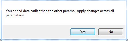
Figure 37 Message from EE.
4. Copy and paste into the form for the time and Diatom diatom algae data as shown in Figure 38
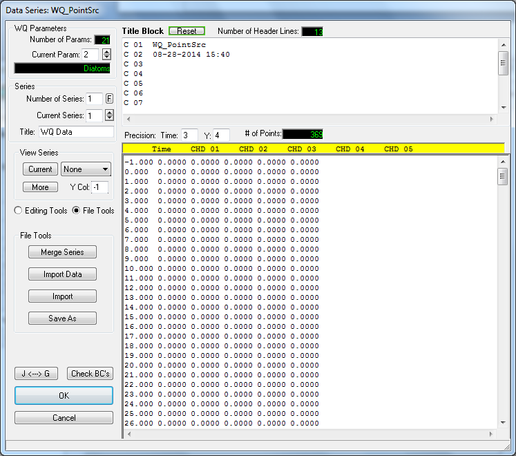
Figure 38 Boundary Condition Settings: Diatom algae Data Series.
...

Figure 47 Boundary Condition Settings: Refractory part. Org. particulate organic nitrogen.

Figure 48 Boundary Condition Settings: Labile part. particulate organic nitrogen.
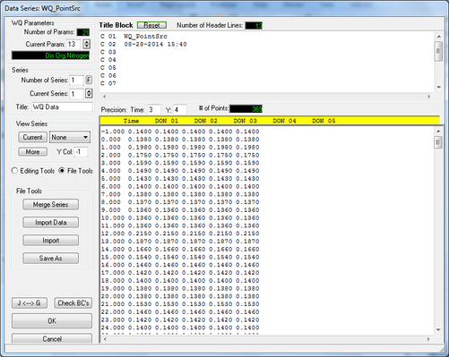
Figure 49 Boundary Condition Settings: Dissolved organic nitrogen.
...
3. From Sediment Diagenesis Option & Parameters form (Figure 59), in the top frame, Benthic Nutrient Flux Method select Spatially & Temporally Constant; enter the values of parameters in the Constant Benthic Flux Rates frame as shown in Figure 60.
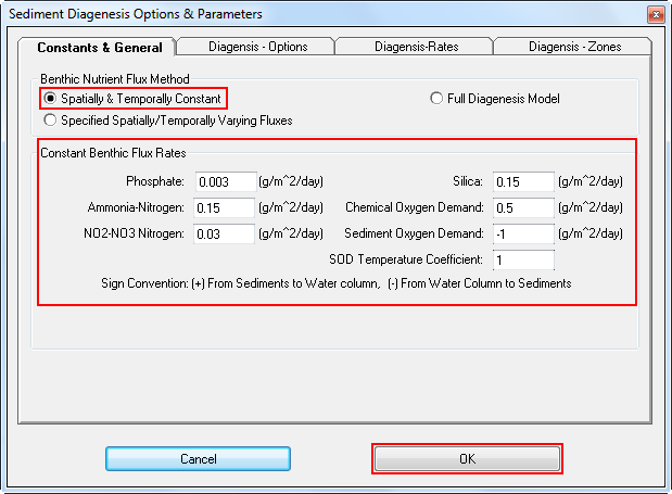
Figure 60 Set Benthic Flux Rates.
...