1 Introduction
...
4. RMC (Right Mouse Click) on the Bounding Polygons blank to open a pop-up menu. In the pop-up menu, select Add Files to browse the polygon file. The land-boundary of the lake will be loaded here.
| Info |
|---|
The polygon file for this model is "Outline.p2d" and can be found in Data/Bathymetry folder of the Demonstration Models provided above. |
| Anchor | ||||
|---|---|---|---|---|
|
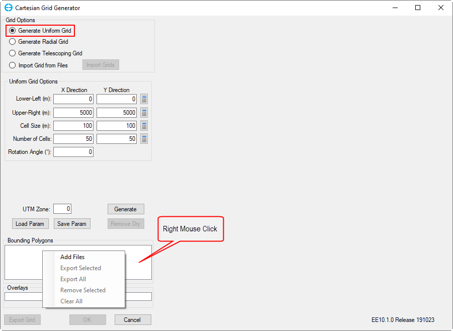
Figure 3. Add polygon file
...
3 Assigning the Initial Conditions
This section will guide you on how to assign the initial conditions, such as the bathymetry, water level, and bottom roughness.
Anchor Figure 6 Figure 6
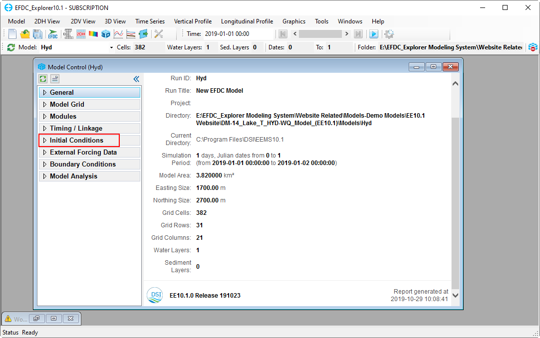
Figure 6. Assigning initial conditions.
3.1 Assigning the Initial Bathymetry
1. Select the Initial Conditions tab and right mouse click (RMC) on the Bathymetry sub-tab. A new Bathymetry form will appear. In that form, click on Assign to define bathymetric value.
Anchor Figure 7 Figure 7
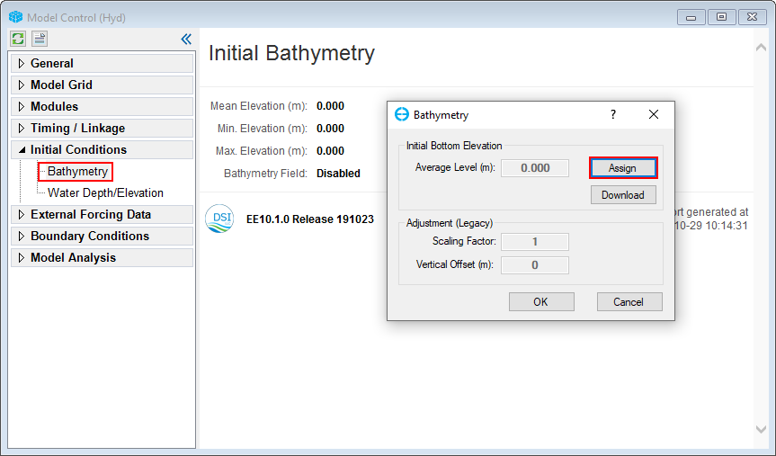
Figure 7. Assigning bathymetry conditions.
2. The area the user wants to assign the bathymetry data to is set by a poly file. In this case, choose All grid cells
3. The data for bathymetry values are assigned by “Bathymetry.dat” file in Bathymetry folder . This bathymetry file is simply an xyz format.
4. Choose Scatter (XYZ) data and then Add file to browse for “Bathymetry.dat”.
Anchor Figure 8 Figure 8
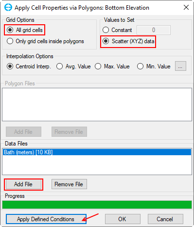
Figure 8. Assigning bathymetry.
5. After adding the data file, click on the Apply Defined Conditions button to make your changes take effect before selecting the OK button.
Anchor Figure 9 Figure 9
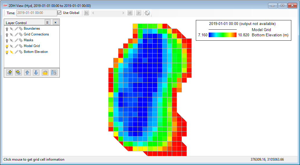
Figure 9. 2DH View of bottom elevation after assigning bathymetry.
...
1. Select Timing/ Linkage tab and RMC on Timing button (Figure 5‑1)
2. Enter the duration of start/ end of the simulation. Note that the boundaries time series should always cover this simulation duration period. Otherwise, the model will not run.
...
Figure 24. Model run time.
Anchor Table 1 Table 1
| Terms | Description |
|---|---|
| Reference Date/Time | The base date of all data and the simulation period. |
| Start Date/Time | The model starts the simulation at that time. |
| End Date/Time | The model stops the simulation at that time. |
| Time of Start (Days) | Number of Julian days after the base date at which to start the simulation. |
| Number of Reference Periods | Total simulation time as a multiple of reference periods. |
| Duration of Reference Period (hours) | The reference period is usually 24 hours; however, it can be set to another value if required. |
| Time Step (seconds) | Also called Delta T, the EFDC model simulation time step. |
| Safety Factor | 0 is a fixed time step. Set 0< safety factor <1 to activate the dynamic time step feature. |
| # Ramp-Up Loops | Number of initial iterations to hold the time step to a constant during ramp-up. |
| Maximum dH/dT | If >0, it is an additional criteria for determining the dynamic time step. |
| Growth Step | The minimum number of iterations for each time step before increasing the time step for the dynamic time stepping |
| Maximum Time Step | This is a maximum-time step |
4. RMC on Linkage button and set Link EFDC Results to EFDC+ Explorer and set Linkage Output Frequency to 60 minutes. This means that EFDC will record the output every 60 minutes for the to display of the model results in the EE. (Figure 5‑225). Note that a smaller output frequency will create a larger output file.
| Anchor | ||||
|---|---|---|---|---|
|
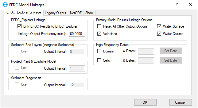
Figure 5‑225. Setting linkage output frequency.
...
This section will guide the user on how to set the hydrodynamic model for the EFDC model’s application of the wet and dry conditions to optimize the simulation time. For this condition, we should make the following settings:
...
3. Enter values for the Dry Depth and the Wet Depth. Then click OK button. Note that the wet depth should always be greater than the dry depth. (Figure 6‑126).
| Anchor | ||||
|---|---|---|---|---|
|
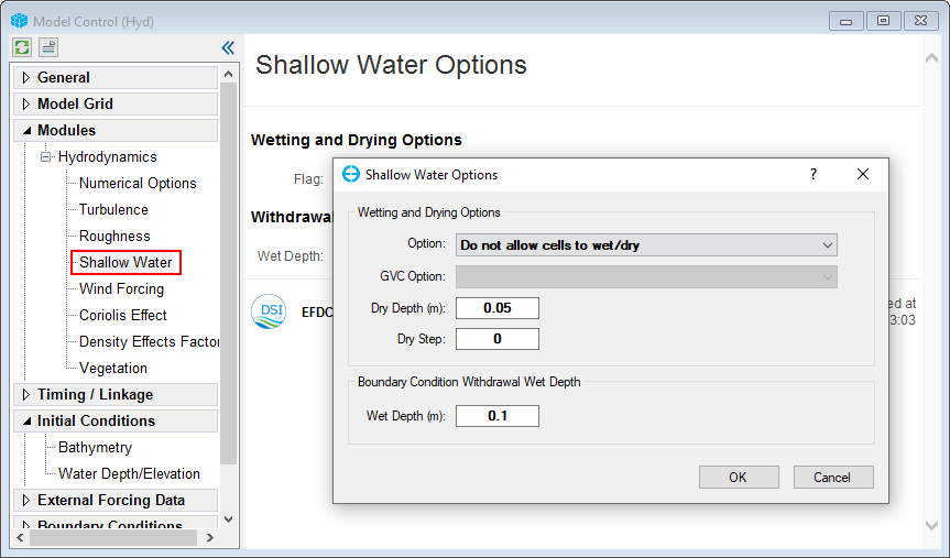
Figure 6‑126. Hydrodynamic model setup.
...
4. Return to select Model Grid tab, RMC on Grid sub-tab and enter the number of vertical layers required into the box. In this case, we will set the vertical layers equal to 5 (Figure 6‑227). Click OK button.
5. Save the model.
Anchor Figure 6-227 Figure 6-227
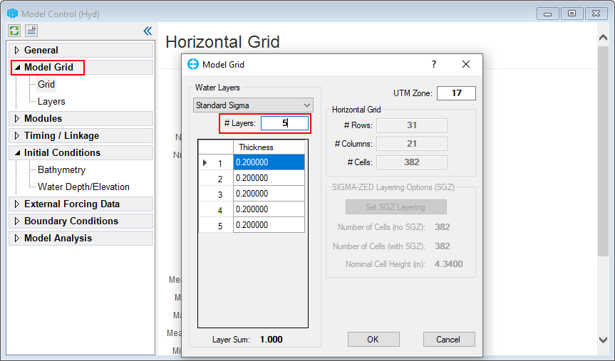
Figure 6‑227. Setting the vertical layers
...
1. Click the Run EFDC icon ![]() on the main form form
on the main form form
Anchor Figure 28 Figure 28
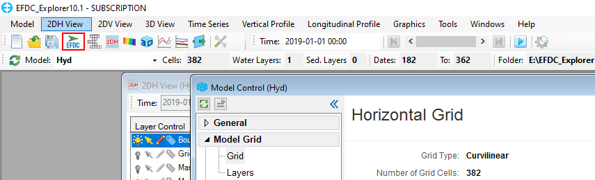
Figure 7‑128. Run EFDC+.
2. Select the Browse icon next to the Executable text box to browse to the EFDC executable file (Figure 7‑229) as default, the EFDC+ executable file is located in the EEMS installation folder (e.g. C:\Program Files\DSI\EEMS10.3)
...
3. Click the Run EFDC+ button to run the model (Figure 7‑229).
Anchor Figure 29 Figure 29
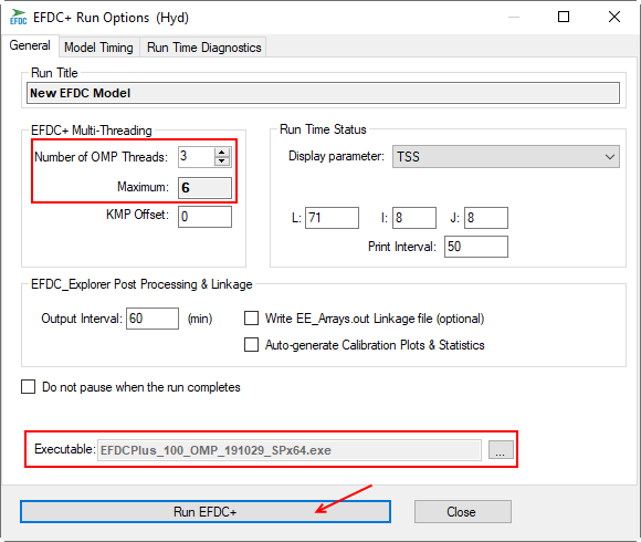
Figure 7‑229. Browse to the EFDC+ executable file.
...
If all settings are correct, the model will start running, and you will see the MS-DOS Window appear showing the model results as shown in Figure 7‑330.
| Info |
|---|
Note that you can press any characters on the keyboard to pause the simulation and You can check the model results . If you want to exit while the simulation hit the same key again, if you want to continue run then hit any other key. |
...
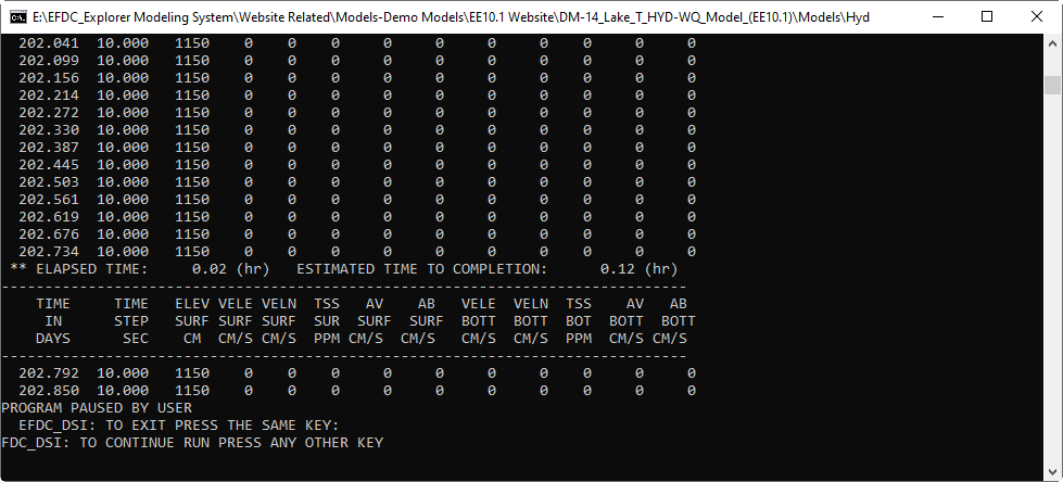
Figure 7‑3. EFDC+ run window.
| Info |
|---|
Note that the user needs to click on the Refresh Model Output button |

| Anchor | ||||
|---|---|---|---|---|
|
Figure 30. EFDC+ run window.
8 Visualizing the EFDC Model Output
This session will teach you how to view the model simulation results. Once the model simulation is completed, click the Refresh Output ![]() button in the toolbar to load the model outputs. These three icons
button in the toolbar to load the model outputs. These three icons  on EE’s main form (Figure 1‑11) are used to view the model simulation results in 2DH View, 2DV View or 3D View, respectively.
...
2. In View Layer Control, select Add a New EFDC View Layer (3407876Figure 31). The user should see View Options window with Primary Group and Parameter to display.
3. Figure 8‑232 is an example of showing the vector and magnitude velocity field results. Similarly, the user can select other parameters to show the model results.
4. Right mouse-click on the Velocity vector layer to modify the vector arrow sample or change the vector color and scale factor (See 3407876 Figure 32)
| Anchor | ||||
|---|---|---|---|---|
|
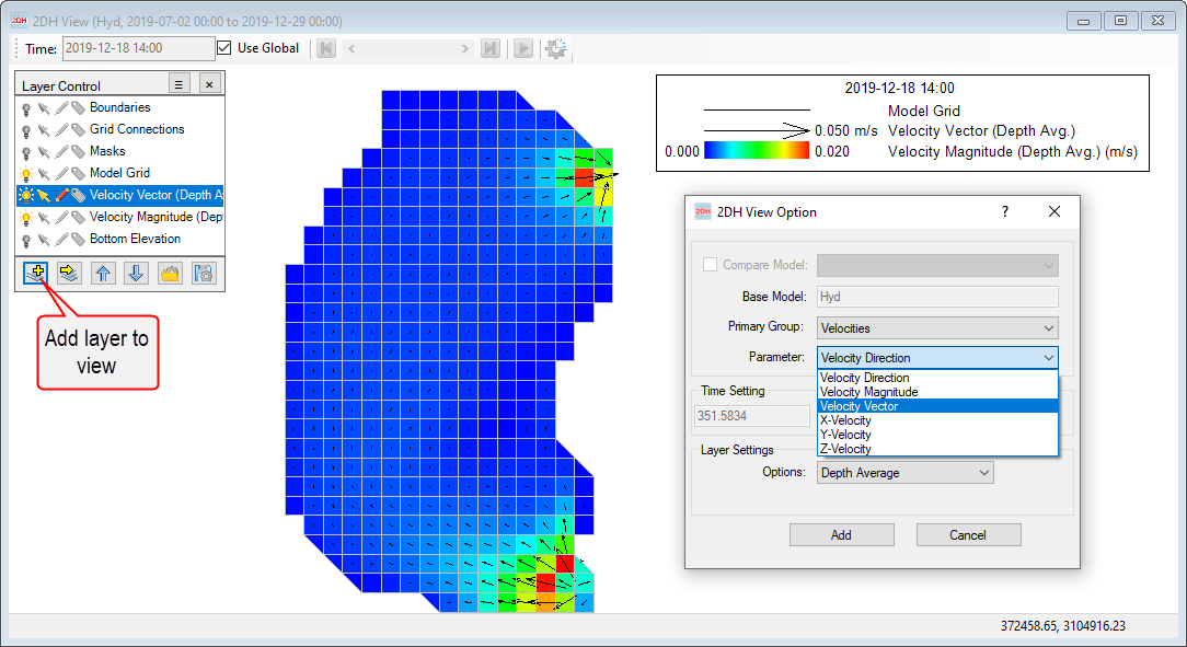
Figure 8‑131. View Layer Control and View Options.
| Anchor | ||||
|---|---|---|---|---|
|
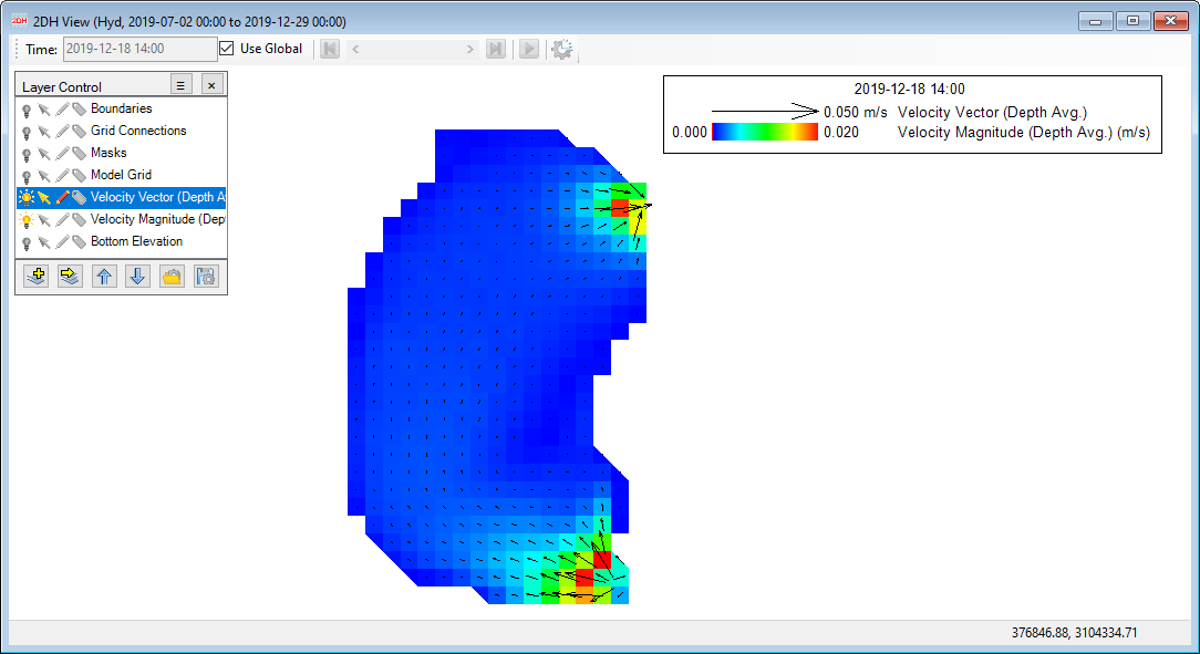
Figure 8‑232. Visualizing the EFDC model output.
...