Bieberbach, L. (1964). "Conformal mapping (4th ed.)", Chelsea: New York, pp. 1–9, chap. 1.
Craig Paul M. and Chung D H "A Simple Algorithm for Grid Generation Based on Laplace Equations" [Report]. - 2012
Fornberg, B. (1980). "A numerical method for conformal mapping", Journal on Scientific and Statistical Computing, 1, pp.386–400.
He Hong, Fan Jian-ren and Cen Ke-fa, (2000). "A numerical method for orthogonal grid generation by Laplace system", Journal of Zhejiang University (Science), Vol. 1, No.2, pp. 125-128.
Hoffman, J.D. (2001). Numerical Methods for Engineers and Scientists, McGraw-Hill International Edition.
Hung Lee Nguyen, (1989). "On the applications of algebraic grid generation methods based on transfinite interpolation", NASA Technical Memorandum 102095, pp.1-23.
Jeng, Y. N., Shu, Y. L, and Lin, W. W. (1995). "On grid generation for internal flow problems by methods solving hyperbolic equations", Numerical heat transfer. Part B 27, pp. 43-61.
Patrick Knup and Stanly Steinberg, (1994). Fundamentals of grid generation, CRC Press
Reese L. Sorenson Joseph L. Steger, ![]() . "Numerical generation of two-dimensional grids by the use of Poisson equations with grid control at boundaries", N81-14722, pp. 449 – 461.
. "Numerical generation of two-dimensional grids by the use of Poisson equations with grid control at boundaries", N81-14722, pp. 449 – 461.
Shih, T. I-P., Bailey, R. T., Nguyen, H. L., & Roelke, R. J. (1991). Algebraic grid generation for complex geometries. International Journal for Numerical Methods in Fluids, 13, 1–31.
Smith, R. E., Kudlimski, R. A., Verton, E. L. E., and Wiese, M. R. (1987). "Algebraic grid Generation", Computer Methods in Appl. Mech. and Eng. 64, pp. 285-300.
Thompson, J. F., Thames, F. C., and Mastin, C. W., (1974). "Automatic numerical generation of body-fitted curvilinear coordinates for a field containing any number of arbitrary 2-D bodies", Journal of Computational Physics, 15(3), pp. 30 - 37.
Thompson, J.F., Soni, B.K. and Weatherill, N.P. (1999). Handbook of Grid generation, CRC Press LLC
Vladimir D. Liseikin (2010). Grid generation methods, Springer
Yuan Chang Liou and Yih Nen Jeng, (1996). "A transfinite interpolation method of grid generation based on multipoints", Journal of Scientific Computing, Vol. 13, No. 1, pp. 105-114.
APPENDIX A
CVLGrid File Formats
Data Format A-1 P2D Polyline/Polygon File
Multiple polylines/polygons can be stored in the same P2D file. The file begins with row 1 that provides the name of the file. The following rows are composed of two columns. The left hand column identifies the X coordinates and the right hand column identifies the Y coordinates. If the file is 3D there will be a third column that represents the Z axis. Each row represents a point on the polyline/polygon. The end of a polyline/polygon is signified by an asterisk ![]() .
.
Example
------------------------
NAME=river
583267.32 2332377.109
583638.541 2332353.487
583787.451 2332360.942
583990.344 2332344.065
584158.122 2332338.04
584258.266 2332337.64
… …
… …
583050.826 2332375.145
583150.712 2332375.089
583215.846 2332385.467
*
NAME=Island
586337.389 2332375.958
586286.096 2332384.429
586148.2 2332412.04
586042.73 2332444.751
… …
… …
*
Data Format A-2 Spline File
The spline file that CVLGrid generates contains the coordinate information for all the splines currently in the workspace. The first two columns provide file information followed by coordinate system type. For CVLGrid all coordinates will be Cartesian. The coordinates for each spline are preceded by two rows. The first row "S #" is the spline number and the second row indicates the number of points in the spline followed by the dimension (2 columns = 2D). The numbers that follow are the coordinates of the spline points. The first column represents the X coordinate and the second point represents the Y coordinate.
*
- DSI Grid generation
- File creation date: 02-Jul-2013 10:47
* - Coordinate System = Cartesian
*
S 1
10 2
-85.123 299.080
-16.104 351.227
91.258 401.840
236.963 414.110
… …
… …
S 2
9 2
-151.074 664.110
-60.583 720.859
137.270 776.074
… …
… …
S 3
2 2
-138.804 730.061
-13.037 303.681
S 4
2 2
1051.380 720.859
1259.969 351.227
Data Format A-3 CVL Grid File
* - DSI CVLGrid Version 1.1
* - The 1st line: CVLGrid file format version
- The 2nd line: # row, # col, coordinate system (0-Cartesian),
- UTM zone (default 0, > 0 for northern hemisphere, < 0 * for southern hemisphere),
- 3 parameters (scale and shift for X and Y, default 1, * 0, 0),
- 2 parameters (scale and shift, default 1 and 0) for
- vertical units conversion Z.
- Other lines: I, J (corner nodes), Cell Type, X, Y, Z corner co-ord
CVLGridFormat=1.0
21 21 0 0 1 0 0 1 0
1 1 5 5.614220639170660E+05 3.697761609812420E+06
1 2 5 5.614094756223090E+05 3.697770022252650E+06
1 3 5 5.613951408251970E+05 3.697779601836410E+06
1 4 5 5.613811567605420E+05 3.697788947034500E+06
1 5 5 5.613674849040790E+05 3.697798083591720E+06
1 6 5 5.613543006637220E+05 3.697806894287380E+06
1 7 5 5.613410426823790E+05 3.697815754262280E+06
1 8 5 5.613279845603650E+05 3.697824480676230E+06
1 9 5 5.613151469448170E+05 3.697833059731270E+06
1 10 5 5.613025568625900E+05 3.697841473366020E+06
APPENDIX B
Mathematical Basis of CVLGrid
As mentioned previously, the Laplace equations are used by CVLGrid for grid generation. Therefore the family of orthogonal curves in a physical domain must be determined:
 (1)
(1)
They must satisfy the Laplace equations:
 (2)
(2)
 ,
,  (3)
(3)
and the Dirichlet boundary conditions:
 ,
,  (4)
(4)
in which Ω is the physical domain with the closed boundary Г. Since this domain is not rectangular, the equations are converted into the logical domain D of the rectangle. The family of orthogonal curves must then be determined:
 (5)
(5)
So that they satisfy the Laplace equations in the logical domain D:
 (6)
(6)
 ,
,  (7)
(7)
 ,
,  ,
, 

with the boundary conditions on four sides of rectangle D:
 ,
,  (8)
(8)
 ,
,  (9)
(9)
 ,
,  (10)
(10)
 ,
,  (11)
(11)
in which are the coordinates in physical space and being dependent variables,
  the coordinates in the logical space D,
  are given values on the boundaries.
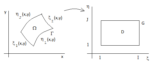
Figure 8 1 Sketches of physical and logical domainsAnchor _Toc454550485 _Toc454550485
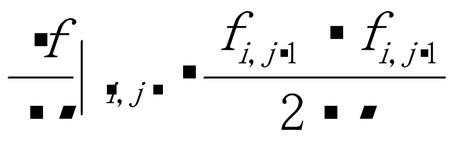
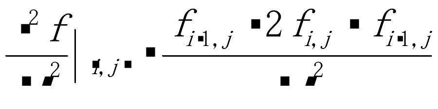
The formulas of the scheme of central space difference for 9 points:
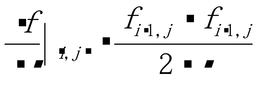 ,
,  (12)
(12)
 ,
, 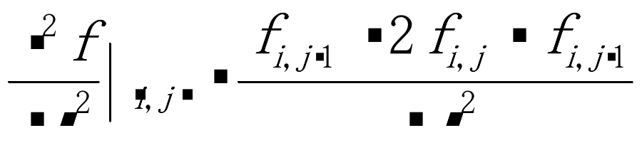 (13)
(13)
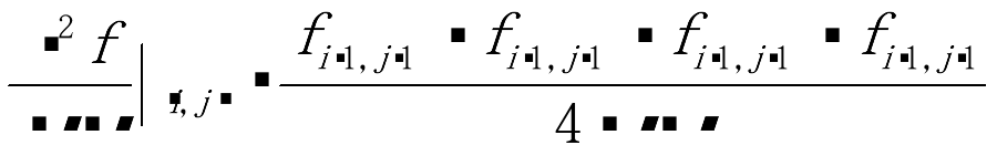 (14)
(14)
Substituting the formulas (12)(14) into Equations (6)(7) we have the formulas of iteration solutions based on SOR method:
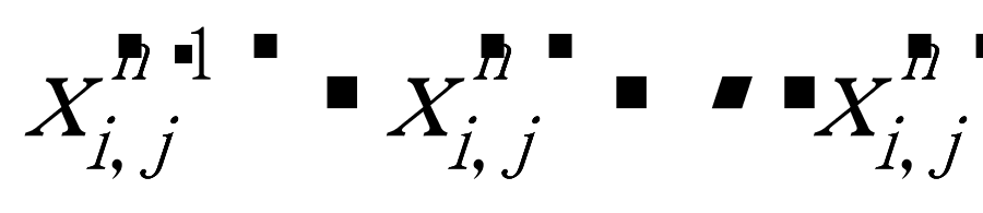 (15)
(15)
 (16)
(16)
in which are known values at the previous iteration,
  depend on
  of 9 points (i, j),
 is the over-relaxation factor, the value of which is a constant,
 .
.
The initial values for the interiors of grid can be directly obtained from transfinite interpolation based on the data sets of given boundary points (x, y).
For a rectangular domain D the optimum value of the over-relaxation factor is determined by Frankel's formula (Hoffman, J.D., 2001) as follows:
 (17)
(17)
 ,
, 
The solutions of x and y are obtained when the following conditions are satisfied:
 and
and  (18)
(18)
Then we have:
 and
and